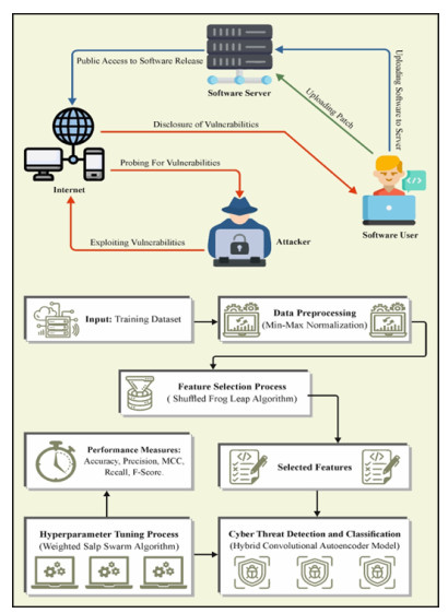
The fast development of the internet of things has been associated with the complex worldwide problem of protecting interconnected devices and networks. The protection of cyber security is becoming increasingly complicated due to the enormous growth in computer connectivity and the number of new applications related to computers. Consequently, emerging intrusion detection systems could execute a potential cyber security function to identify attacks and variations in computer networks. An efficient data-driven intrusion detection system can be generated utilizing artificial intelligence, especially machine learning methods. Deep learning methods offer advanced methodologies for identifying abnormalities in network traffic efficiently. Therefore, this article introduced a weighted salp swarm algorithm with deep learning-powered cyber-threat detection and classification (WSSADL-CTDC) technique for robust network security, with the aim of detecting the presence of cyber threats, keeping networks secure using metaheuristics with deep learning models, and implementing a min-max normalization approach to scale the data into a uniform format to accomplish this. In addition, the WSSADL-CTDC technique applied the shuffled frog leap algorithm (SFLA) to elect an optimum subset of features and applied a hybrid convolutional autoencoder (CAE) model for cyber threat detection and classification. A WSSA-based hyperparameter tuning method can be employed to enhance the detection performance of the CAE model. The simulation results of the WSSADL-CTDC system were examined in the benchmark dataset. The extensive analysis of the accuracy of the results found that the WSSADL-CTDC technique exhibited a better value of 99.13% than comparable methods on different measures.
Citation: Maha M. Althobaiti, José Escorcia-Gutierrez. Weighted salp swarm algorithm with deep learning-powered cyber-threat detection for robust network security[J]. AIMS Mathematics, 2024, 9(7): 17676-17695. doi: 10.3934/math.2024859
The fast development of the internet of things has been associated with the complex worldwide problem of protecting interconnected devices and networks. The protection of cyber security is becoming increasingly complicated due to the enormous growth in computer connectivity and the number of new applications related to computers. Consequently, emerging intrusion detection systems could execute a potential cyber security function to identify attacks and variations in computer networks. An efficient data-driven intrusion detection system can be generated utilizing artificial intelligence, especially machine learning methods. Deep learning methods offer advanced methodologies for identifying abnormalities in network traffic efficiently. Therefore, this article introduced a weighted salp swarm algorithm with deep learning-powered cyber-threat detection and classification (WSSADL-CTDC) technique for robust network security, with the aim of detecting the presence of cyber threats, keeping networks secure using metaheuristics with deep learning models, and implementing a min-max normalization approach to scale the data into a uniform format to accomplish this. In addition, the WSSADL-CTDC technique applied the shuffled frog leap algorithm (SFLA) to elect an optimum subset of features and applied a hybrid convolutional autoencoder (CAE) model for cyber threat detection and classification. A WSSA-based hyperparameter tuning method can be employed to enhance the detection performance of the CAE model. The simulation results of the WSSADL-CTDC system were examined in the benchmark dataset. The extensive analysis of the accuracy of the results found that the WSSADL-CTDC technique exhibited a better value of 99.13% than comparable methods on different measures.

| [1] |
M. A. Ferrag, O. Friha, L. Maglaras, H. Janicke, L. Shu, Federated deep learning for cyber security in the internet of things: Concepts, applications, and experimental analysis, IEEE Access, 9 (2021), 138509–138542. https://doi.org/10.1109/ACCESS.2021.3118642 doi: 10.1109/ACCESS.2021.3118642

|
| [2] |
Y. Li, Y. Zuo, H. Song, Z. Lv, Deep learning in security of internet of things, IEEE Internet Things J., 9 (2022), 22133–22146. https://doi.org/10.1109/JIOT.2021.3106898 doi: 10.1109/JIOT.2021.3106898
|
| [3] | A. Salih, S. T. Zeebaree, S. Ameen, A. Alkhyyat, H. M. Shukur, A survey on the role of artificial intelligence, machine learning and deep learning for cybersecurity attack detection, In: 2021 7th International engineering conference"Research & innovation amid global pandemic" (IEC), IEEE, 2021, 61–66. https://doi.org/10.1109/IEC52205.2021.9476132 |
| [4] |
Z. Z. Xian, F. Zhang, Image real-time detection using LSE-Yolo neural network in artificial intelligence-based internet of things for smart cities and smart homes, Wirel. Commun. Mob. Com., 2022 (2022), 2608798. https://doi.org/10.1155/2022/2608798 doi: 10.1155/2022/2608798
|
| [5] |
A. D. Raju, I. Y. Abualhaol, R. S. Giagone, Y. Zhou, S. Huang, A survey on cross-architectural IoT malware threat hunting, IEEE Access, 9 (2021), 91686–91709. https://doi.org/10.1109/ACCESS.2021.3091427 doi: 10.1109/ACCESS.2021.3091427
|
| [6] |
B. Jothi, M. Pushpalatha, Wils-trs—A novel optimized deep learning based intrusion detection framework for IoT networks, Pers. Ubiquit. Comput., 27 (2023), 1285–1301. https://doi.org/10.1007/s00779-021-01578-5 doi: 10.1007/s00779-021-01578-5
|
| [7] |
P. Dixit, S. Silakari, Deep learning algorithms for cybersecurity applications: A technological and status review, Comput. Sci. Rev., 39 (2021), 100317. https://doi.org/10.1016/j.cosrev.2020.100317 doi: 10.1016/j.cosrev.2020.100317
|
| [8] |
D. Chen, P. Wawrzynski, Z. Lv, Cyber security in smart cities: A review of deep learning-based applications and case studies, Sustain. Cities Soc., 66 (2021), 102655. https://doi.org/10.1016/j.scs.2020.102655 doi: 10.1016/j.scs.2020.102655
|
| [9] |
R. Ahmad, I. Alsmadi, Machine learning approaches to iot security: A systematic literature review, Internet Things, 14 (2021), 100365. https://doi.org/10.1016/j.iot.2021.100365 doi: 10.1016/j.iot.2021.100365
|
| [10] |
E. Bout, V. Loscri, A. Gallais, How machine learning changes the nature of cyberattacks on iot networks: A survey, IEEE Commun. Surv. Tutor., 24 (2022), 248–279. https://doi.org/10.1109/COMST.2021.3127267 doi: 10.1109/COMST.2021.3127267
|
| [11] |
E. H. Houssein, D. Oliva, N. A. Samee, N. F. Mahmoud, M. M. Emam, Liver cancer algorithm: A novel bio-inspired optimizer, Comput. Biol. Med., 165 (2023), 107389. https://doi.org/10.1016/j.compbiomed.2023.107389 doi: 10.1016/j.compbiomed.2023.107389
|
| [12] |
S. Li, H. Chen, M. Wang, A. A. Heidari, S. Mirjalili, Slime mould algorithm: A new method for stochastic optimization, Future Gener. Comp. Syst., 111 (2020), 300–323. https://doi.org/10.1016/j.future.2020.03.055 doi: 10.1016/j.future.2020.03.055
|
| [13] |
X. Zhou, Y. Chen, Z. Wu, A. A. Heidari, H. Chen, E. Alabdulkreem, et al., Boosted local dimensional mutation and all-dimensional neighborhood slime mould algorithm for feature selection, Neurocomputing, 551 (2023), 126467. https://doi.org/10.1016/j.neucom.2023.126467 doi: 10.1016/j.neucom.2023.126467
|
| [14] |
G. Wang, Moth search algorithm: A bio-inspired metaheuristic algorithm for global optimization problems, Memetic. Comp., 10 (2018), 151–164. https://doi.org/10.1007/s12293-016-0212-3 doi: 10.1007/s12293-016-0212-3
|
| [15] |
Y. Yang, H. Chen, A. A. Heidari, A. H. Gandomi, Hunger games search: Visions, conception, implementation, deep analysis, perspectives, and towards performance shifts, Expert Syst. Appl., 177 (2021), 114864. https://doi.org/10.1016/j.eswa.2021.114864 doi: 10.1016/j.eswa.2021.114864
|
| [16] |
J. C. Butcher, G. Wanner, Runge-kutta methods: Some historical notes, Appl. Numer. Math., 22 (1996), 113–151. https://doi.org/10.1016/S0168-9274(96)00048-7 doi: 10.1016/S0168-9274(96)00048-7
|
| [17] | J. Tu, H. Chen, M. Wang, A. H. Gandomi, The colony predation algorithm, J. Bionic Eng., 18 (2021), 674–710. |
| [18] |
I. Ahmadianfar, A. A. Heidari, S. Noshadian, H. Chen, A. H. Gandomi, INFO: An efficient optimization algorithm based on weighted mean of vectors, Expert Syst. Appl., 195 (2022), 116516. https://doi.org/10.1016/j.eswa.2022.116516 doi: 10.1016/j.eswa.2022.116516
|
| [19] |
A. A. Heidari, S. Mirjalili, H. Faris, I. Aljarah, M. Mafarja, H. Chen, Harris hawks optimization: Algorithm and applications, Future Gener. Comp. Syst., 97 (2019), 849–872. https://doi.org/10.1016/j.future.2019.02.028 doi: 10.1016/j.future.2019.02.028
|
| [20] |
H. Su, D. Zhao, A. A. Heidari, L. Liu, X. Zhang, M. Mafarja, et al., RIME: A physics-based optimization, Neurocomputing, 532 (2023), 183–214. https://doi.org/10.1016/j.neucom.2023.02.010 doi: 10.1016/j.neucom.2023.02.010
|
| [21] |
Y. Li, D. Zhao, C. Ma, J. Escorcia-Gutierrez, N. O. Aljehane, X. Ye, CDRIME-MTIS: An enhanced rime optimization-driven multi-threshold segmentation for covid-19 X-ray images, Comput. Biol. Med., 169 (2024), 107838. https://doi.org/10.1016/j.compbiomed.2023.107838 doi: 10.1016/j.compbiomed.2023.107838
|
| [22] |
A. Yazdinejad, M. Kazemi, R. M. Parizi, A. Dehghantanha, H. Karimipour, An ensemble deep learning model for cyber threat hunting in industrial internet of things, Digit. Commun. Netw., 9 (2023), 101–110. https://doi.org/10.1016/j.dcan.2022.09.008 doi: 10.1016/j.dcan.2022.09.008
|
| [23] |
I. A. Khan, N. Moustafa, D. Pi, K. M. Sallam, A. Y. Zomaya, B. Li, A new explainable deep learning framework for cyber threat discovery in industrial iot networks, IEEE Internet Things J., 9 (2022), 11604–11613. https://doi.org/10.1109/JIOT.2021.3130156 doi: 10.1109/JIOT.2021.3130156
|
| [24] |
I. Bibi, A. Akhunzada, N. Kumar, Deep AI-powered cyber threat analysis in IIOT, IEEE Internet Things J., 10 (2023), 7749–7760. https://doi.org/10.1109/JIOT.2022.3229722 doi: 10.1109/JIOT.2022.3229722
|
| [25] | S. Das, Y. Manchala, S. K. Rout, S. K. Panda, Deep learning and metaheuristics based cyber threat detection in internet of things enabled smart city environment, 2023. http://dx.doi.org/10.21203/rs.3.rs-3141258/v1 |
| [26] | R. Wei, L. Cai, L. Zhao, A. Yu, D. Meng, DeepHunter: A graph neural network based approach for robust cyber threat hunting, In: Security and privacy in communication networks, Springer, 398 (2021), 3–24. https://doi.org/10.1007/978-3-030-90019-9_1 |
| [27] |
A. N. Ndife, Y. Mensin, W. Rakwichian, P. Muneesawang, Cyber-security audit for smart grid networks: An optimized detection technique based on bayesian deep learning, J. Internet Serv. Inf. Secur., 12 (2022), 95–114. https://dx.doi.org/10.22667/JISIS.2022.05.31.095 doi: 10.22667/JISIS.2022.05.31.095
|
| [28] | M. A. Ferrag, D. Hamouda, M. Debbah, L. Maglaras, A. Lakas, Generative adversarial networks-driven cyber threat intelligence detection framework for securing internet of things, In: 2023 19th International conference on distributed computing in smart systems and the internet of things (DCOSS-IoT), IEEE, 2023,196–200. https://doi.org/10.1109/DCOSS-IoT58021.2023.00042 |
| [29] | T. Elangovan, S. Sukumaran, S. Muthumarilakshmi, An efficient recurrent neural network based classification method for cyber threat detection analysis, J. Alebr. Stat., 13 (2022), 5514–5520. |
| [30] |
Y. Zhou, B. Yang, H. Hou, L. Zhang, T. Wang, M. Hu, Continuous leakage-resilient identity-based encryption with tight security, Comput. J., 62 (2019), 1092–1105. https://doi.org/10.1093/comjnl/bxy144 doi: 10.1093/comjnl/bxy144
|
| [31] |
J. Xu, S. H. Park, X. Zhang, A bio-inspired motion sensitive model and its application to estimating human gaze positions under classified driving conditions, Neurocomputing, 345 (2019), 23–35. https://doi.org/10.1016/j.neucom.2018.09.093 doi: 10.1016/j.neucom.2018.09.093
|
| [32] |
Y. Li, W. G. Cui, H. Huang, Y. Z. Guo, K. Li, T. Tan, Epileptic seizure detection in EEG signals using sparse multiscale radial basis function networks and the fisher vector approach, Knowledge Based Syst., 164 (2019), 96–106. https://doi.org/10.1016/j.knosys.2018.10.029 doi: 10.1016/j.knosys.2018.10.029
|
| [33] |
Y. Chen, L. Feng, C. Zheng, T. Zhou, L. Liu, P. Liu, et al., LDANet: Automatic lung parenchyma segmentation from CT images, Comput. Biol. Med., 155 (2023), 106659. https://doi.org/10.1016/j.compbiomed.2023.106659 doi: 10.1016/j.compbiomed.2023.106659
|
| [34] |
S. B. Lin, Generalization and expressivity for deep nets, IEEE Trans. Neural Netw. Learn. Syst., 30 (2019), 1392–1406. https://doi.org/10.1109/TNNLS.2018.2868980 doi: 10.1109/TNNLS.2018.2868980
|
| [35] |
Q. Pham, B. Mohammadi, R. Moazenzadeh, S. Heddam, R. P. Zolá, A. Sankaran, et al., Prediction of lake water-level fluctuations using adaptive neuro-fuzzy inference system hybridized with metaheuristic optimization algorithms, Appl. Water Sci., 13 (2023), 13. https://doi.org/10.1007/s13201-022-01815-z doi: 10.1007/s13201-022-01815-z
|
| [36] |
R. Dash, R. Dash, R. Rautray, An evolutionary framework-based microarray gene selection and classification approach using binary shuffled frog leaping algorithm, J. King Saud Univ. Comput. Inf. Sci., 34 (2022), 880–891. https://doi.org/10.1016/j.jksuci.2019.04.002 doi: 10.1016/j.jksuci.2019.04.002
|
| [37] |
M. Mafarja, T. Thaher, M. A. Al-Betar, J. Too, M. A. Awadallah, I. A. Doush, et al., Classification framework for faulty software using enhanced exploratory whale optimizer-based feature selection scheme and random forest ensemble learning, Appl. Intell., 53 (2023), 18715–18757. https://doi.org/10.1007/s10489-022-04427-x doi: 10.1007/s10489-022-04427-x
|
| [38] |
P. Bedi, P. Gole, Plant disease detection using hybrid model based on convolutional autoencoder and convolutional neural network, Artif. Intell. Agric., 5 (2021), 90–101. https://doi.org/10.1016/j.aiia.2021.05.002 doi: 10.1016/j.aiia.2021.05.002
|
| [39] |
M. A. Syed, R. Syed, Weighted salp swarm algorithm and its applications towards optimal sensor deployment, J. King Saud Univ. Comput. Inf. Sci., 34 (2022), 1285–1295. https://doi.org/10.1016/j.jksuci.2019.07.005 doi: 10.1016/j.jksuci.2019.07.005
|
| [40] |
G. D. Singh, V. Tripathi, A. Dumka, R. S. Rathore, M. Bajaj, J. Escorcia-Gutierrez, et al., A novel framework for capacitated sdn controller placement: Balancing latency and reliability with pso algorithm, Alex. Eng. J., 87 (2024), 77–92. https://doi.org/10.1016/j.aej.2023.12.018 doi: 10.1016/j.aej.2023.12.018
|
| [41] |
Y. Meidan, M. Bohandana, Y. Mathov, Y. Mirsky, A. Shabtai, D. Breitenbacher, et al., N-BaIoT—Network-based detection of IoT botnet attacks using deep autoencoders, IEEE Pervas. Comput., 17 (2018), 12–22. https://doi.org/10.1109/MPRV.2018.03367731 doi: 10.1109/MPRV.2018.03367731
|
| [42] |
F. Alrowais, S. Althahabi, S. S. Alotaibi, A. Mohamed, M. A. Hamza, R. Marzouk, Automated machine learning enabled cyber security threat detection in the internet of things environment, Comput. Syst. Sci. Eng., 45 (2023), 687–700. https://doi.org/10.32604/csse.2023.030188 doi: 10.32604/csse.2023.030188
|
| [43] |
N. Savanović, A. Toskovic, A. Petervoic, M. Zivkovic, R. Damaševičius, L. Jovanovic, Intrusion detection in healthcare 4.0 internet of things systems via metaheuristics optimized machine learning, Sustainability, 15 (2023), 12563. https://doi.org/10.3390/su151612563 doi: 10.3390/su151612563
|
| [44] |
S. S. Kareem, R. R. Mostafa, F. A. Hashim, H. M. El-Bakry, An effective feature selection model using hybrid metaheuristic algorithms for IoT intrusion detection, Sensors, 22 (2022), 1396. https://doi.org/10.3390/s22041396 doi: 10.3390/s22041396
|


Figures(11) / Tables(5)

Maha M. Althobaiti, José Escorcia-Gutierrez. Weighted salp swarm algorithm with deep learning-powered cyber-threat detection for robust network security[J]. AIMS Mathematics, 2024, 9(7): 17676-17695. doi: 10.3934/math.2024859


 DownLoad: