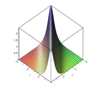
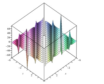
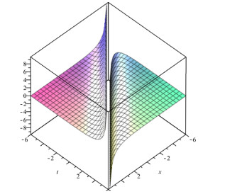
Lie symmetry analysis of differential equations proves to be a powerful tool to solve or atleast to reduce the order and non-linearity of the equation. The present article focuses on the solution of Generalized Equal Width wave (GEW) equation using Lie group theory. Over the years, different solution methods have been tried for GEW but Lie symmetry analysis has not been done yet. At first, we obtain the infinitesimal generators, commutation table and adjoint table of Generalized Equal Width wave (GEW) equation. After this, we find the one dimensional optimal system. Then we reduce GEW equation into non-linear ordinary differential equation (ODE) by using the Lie symmetry method. This transformed equation can take us to the solution of GEW equation by different methods. After this, we get the travelling wave solution of GEW equation by using the Sine-cosine method. We also give graphs of some solutions of this equation.
Citation: Mobeen Munir, Muhammad Athar, Sakhi Sarwar, Wasfi Shatanawi. Lie symmetries of Generalized Equal Width wave equations[J]. AIMS Mathematics, 2021, 6(11): 12148-12165. doi: 10.3934/math.2021705
Lie symmetry analysis of differential equations proves to be a powerful tool to solve or atleast to reduce the order and non-linearity of the equation. The present article focuses on the solution of Generalized Equal Width wave (GEW) equation using Lie group theory. Over the years, different solution methods have been tried for GEW but Lie symmetry analysis has not been done yet. At first, we obtain the infinitesimal generators, commutation table and adjoint table of Generalized Equal Width wave (GEW) equation. After this, we find the one dimensional optimal system. Then we reduce GEW equation into non-linear ordinary differential equation (ODE) by using the Lie symmetry method. This transformed equation can take us to the solution of GEW equation by different methods. After this, we get the travelling wave solution of GEW equation by using the Sine-cosine method. We also give graphs of some solutions of this equation.

| [1] | R. Gilmore, Lie Groups, Physics and Geometry: An Introduction for Physicists, Engineers and Chemists, Cambridge U. Press, New York, 2008. |
| [2] | T. Xiang, A summary of the Korteweg-de Vries equation, 2015. |
| [3] |
H. N. Hassan, H. K. Saleh, The solution of the regularized long wave equation using the fourier Leap-frog method, Z. Naturforsch. A, 65 (2010), 268-276. doi: 10.1515/zna-2010-0402

|
| [4] |
P. J. Morrison, J. D. Meiss, J. R. Cary, Scattering of regularized-long-wave solitary waves, Physica D, 11 (1984), 324-336. doi: 10.1016/0167-2789(84)90014-9
|
| [5] | S. Dhawan, Turgut Ak, G. Apaydin, Algorithms for numerical solution of the Equal Width wave equation using multi-quadric quasi-interpolation method, Int. J. Mod. Phys. C, 30 (2019), 17. |
| [6] |
L. R. T. Gardner, G. A. Gardner, F. A. Ayoub, N. K. Amein, Simulations of the EW undular bore, Commun. Numer. Meth. En., 13 (1997), 583-592. doi: 10.1002/(SICI)1099-0887(199707)13:7<583::AID-CNM90>3.0.CO;2-E
|
| [7] | M. G. Rani, S. Padmasekaran, T. Shanmugapriya, Symmetry reductions of (2+1)-dimensional Equal Width wave equation, Int. J. Appl. Comput. Math., 12 (2017). |
| [8] | A. Esen, A numerical solution of the Equal Width wave equation by a Lumped Galerkin method, Appl. Math. Comput., 168 (2005), 270-282. |
| [9] | B. Saka, A finite element method for Equal Width wave equation, Appl. Math. Comput., 175 (2006), 730-747. |
| [10] | I. Dag, B. Saka, A cubic B-spline collocation method for the EW equation, Math. Comput. Appl., 9 (2004), 381-392. |
| [11] | S. K. Bhowmik, S. B. G.Karakoc, Numerical solutions of the Generalized Equal Width wave equation using Petrov-Galerkin method, Appl. Anal., 100 (2019), 714-734. |
| [12] | R. Arora, M. J. Siddiqui, V. P. Singh, Solution of the Modified Equal Width wave equation, its variant and non-homogeneous Burger's equation by RDT Method, Am. J. Comput. Appl. Math., 1 (2011), 53-56. |
| [13] | S. T. Mohyud-Din, A. Yildirim, M. E. Berberler, M. M. Hosseini, Numerical solution of Modified Equal Width wave equation, World Appl. Sci. J., 8 (2010), 792-798. |
| [14] |
T. Geyikli, S. B. G. Karakoc, Septic B-spline collocation method for the numerical solution of the Modified Equal Width wave equation, Appl. Math., 2 (2011), 739-749. doi: 10.4236/am.2011.26098
|
| [15] |
T. Geyikli, S. B. G. Karakoc, Subdomain finite element method with quartic B-splines for the Modified Equal Width wave equation, Comput. Math. Math. Phys., 55 (2015), 410-421. doi: 10.1134/S0965542515030070
|
| [16] |
M. Merdan, A. Yildirim, A. Gokdogan, Numerical solution of time-fraction Modified Equal Width wave equation, Eng. Comput., 29 (2012), 766-777. doi: 10.1108/02644401211257254
|
| [17] |
A. Esen, A Lumped Galerkin method for the numerical solution of the Modified Equal Width wave equation using quadratic B-splines, Int. J. Comput. Math., 83 (2006), 449-459. doi: 10.1080/00207160600909918
|
| [18] |
B. Saka, Algorithms for numerical solution of the Modified Equal Width wave equation using collocation method, Math. comput. model., 45 (2007), 1096-1117. doi: 10.1016/j.mcm.2006.09.012
|
| [19] | M. Yaseer, A. Essa, Multigrid method for solving the Generalized Equal Width wave equation, Int. J. Math. Arch., 8 (2017). |
| [20] |
K. R. Raslan, Collocation method using cubic B-spline for the Generalized Equal Width wave equation, Int. J. Simul. Process Model., 2 (2006), 37-44. doi: 10.1504/IJSPM.2006.009019
|
| [21] |
N. Taghizadeh, M. Mirzazadeh, M. Akbari, M. Rahimian, Exact soliton solutions for Generalized Equal Width wave equation, Math. Sci. Lett., 2 (2013), 99-106. doi: 10.12785/msl/020204
|
| [22] | H. Zeybek, B. G. Karakoc, Application of the collocation method with B-spline to the GEW equation, Electron. Trans. Numer. Anal., 46 (2017), 71-88. |
| [23] |
T. Roshan, A Petrov-Galerkin method for solving the Generalized Equal Width wave (GEW) equation, J. Comput. Appl. Math., 235 (2011), 1641-1652. doi: 10.1016/j.cam.2010.09.006
|
| [24] |
L. R. T. Gardner, G. A. Gardner, T. Geyikli, The boundary forced MKdV equation, J. Comput. Phys., 113 (1994), 5-12. doi: 10.1006/jcph.1994.1113
|
| [25] | D. Kaya, A numerical simulation of solitary-wave solutions of the generalized regularized long wave equation, Appl. Math. Comput., 149 (2004), 833-841. |
| [26] |
D. Kaya, S. M. El-Sayed, An application of the decomposition method for the Generalized KdV and RLW equations, Chaos Soliton. Fract., 17 (2003), 869-877. doi: 10.1016/S0960-0779(02)00569-6
|
| [27] | S. Kumar, Finite difference method: A brief study, SSRN Elect. J., 6 (2014). |
| [28] |
S. C. Shiralashetti, M. H. Kantli, A. B. Deshi, A new wavelet multigrid method for the numerical solution of elliptic type differential equations, Alex. Eng. J., 57 (2018), 203-209. doi: 10.1016/j.aej.2016.12.007
|
| [29] |
M. N. O. Sadiku, C. N. Obiozor, A simple introduction to the method of lines, Int. J. Elec. Eng. Edu., 37 (2000), 282-296. doi: 10.7227/IJEEE.37.3.8
|
| [30] | V. Dolean, P. Jolivet, F. Nataf, An Introduction to Domain Decomposition Methods: Algorithms, Theory and Parallel Implementation, Siam Press Manag. Co. Ltd., 2016. |
| [31] |
J. Droniou, R. Eymard, T. Gallouet, R. Herbin, The gradient discretisation method for linear advection problems, Comput. Methods Appl. Math., 20 (2020), 437-458. doi: 10.1515/cmam-2019-0060
|
| [32] | Z. Jiang, Lingde Su, T. Jiang, A Meshfree method for numerical solution of non-homogeneous time-dependent problems, Abstr. Appl. Anal., 11 (2014). |
| [33] | N. Rai, S. Mondal, Spectral methods to solve non-linear problems: A review, Part. Diff. Equ. Appl. Math., 4 (2021). |
| [34] | F. Cheng, X. Wang, B. A. Barsky, Quadratic B-spline curve interpolation, Comput. Math., 41 (2001), 39-50. |
| [35] |
Q. Zhao, L. Wu, Darboux transformation and explicit solutions to the generalized TD equation, Appl. Math. Lett., 67 (2017), 1-6. doi: 10.1016/j.aml.2016.11.012
|
| [36] | R. Li, X. Geng, B. Xue, Darboux transformations for a matrix long-wave-short-wave equation and higher-order rational rogue-wave solutions, Appl. Math. Lett., 43 (2020), 948-967. |
| [37] | M. A. Ablowitz, P. A. Clarkson, Solitons, Non-linear Evolution Equations and Inverse Scattering, Cambridge Uni. Press, 1991. |
| [38] | W. X. Ma, Inverse scattering for non-local reverse-time non-linear schrödinger equations, Appl. Math. Lett., 102 (2020). |
| [39] |
F. Mahmud, Md Samsuzzoha, M. A. Akbar, The generalized Kudryashov method to obtain exact traveling wave solutions of the Phi-four equation and the fisher equation, Results Phys., 7 (2017), 4296-4302. doi: 10.1016/j.rinp.2017.10.049
|
| [40] | M. S. Islam, K. Khan, A. H. Arnous, Generalized Kudryashov method for solving some (3+1)-dimensional non-linear evolution equations, New Trend Math. Sci., 3 (2015), 46-57. |
| [41] | T. Motsepa, C. M. Khalique, Conservation laws and solutions of a generalized coupled (2+1)-dimensional Burger's system, Comput. Math., 74 (2017), 1333-1339. |
| [42] |
M. L. Wang, Y. B. Zhou, Z. B. Li, Application of a homogeneous balance method to exact solutions of non-linear equations in mathematical physics, Phys. Lett. A, 216 (1996), 67-75. doi: 10.1016/0375-9601(96)00283-6
|
| [43] | A. M. Wazwaz, The tanh-coth method for solitons and kink solutions for non-linear parabolic equations, Appl. Math. Comput., 188 (2007), 1467-1475. |
| [44] | R. Hirota, The Direct Method in Soliton Theory, Cambridge Uni. Press, 2004. |
| [45] | Z. Y. Zhang, Jacobi elliptic function expansion method for the Modified Korteweg-de Vries-Zakharov-Kuznetsov and the Hirota equations, Phys. Lett. A, 60 (2001), 1384-1394. |
| [46] |
I. Simbanefayi, C. M. Khalique, Travelling wave solutions and conservation laws for the Korteweg-de Vries-Bejamin-Bona-Mahony equation, Results Phys., 8 (2018), 57-63. doi: 10.1016/j.rinp.2017.10.041
|
| [47] |
A. M. Wazwaz, Exact solutions for the ZK-MEW equation by using the tanh and sine$-$cosine methods, Int. J. Comput. Math., 82 (2005), 699-708. doi: 10.1080/00207160512331329069
|
| [48] |
S. Kumar, W. X. Ma, A. Kumar, Lie symmetries, optimal system and group-invariant solutions of the (3+1)-dimensional generalized KP equation, Chin. J. Phys., 69 (2021), 1-23. doi: 10.1016/j.cjph.2020.11.013
|
| [49] | S. Kumar, D. Kumar, A. M. Wazwaz, Lie symmetries, optimal system, group-invariant solutions and dynamical behaviors of solitary wave solutions for a (3+1)-dimensional KdV-type equation, Eur. Phys. J. Plus, 136 (2021). |
| [50] |
S. Kumar, L. Kaur, M. Niwas, Some exact invariant solutions and dynamical structures of multiple solitons for the (2+1)-dimensional Bogoyavlensky-Konopelchenko equation with variable coefficients using Lie symmetry analysis, Chin. J. Phys., 71 (2021), 518-538. doi: 10.1016/j.cjph.2021.03.021
|
| [51] | S. Kumar, M. Niwas, I. Hamid, Lie symmetry analysis for obtaining exact soliton solutions of generalized Camassa-Holm-Kadomtsev-Petviashvili equation, Int. J. Mod. Phys. B, 35 (2021). |
| [52] | H. Liu, J. Li, Lie symmetry analysis and exact solutions for the short pulse equation, non-linear analysis: Theory, methods and applications, Chin. J. of Phys., 71 (2009), 2126-2133. |
| [53] |
A. Chauhan, R. Arora, A. Tomar, Lie symmetry analysis and traveling wave solutions of Equal Width wave equation, Proyecciones, 39 (2020), 179-198. doi: 10.22199/issn.0717-6279-2020-01-0012
|
| [54] |
S. I. Zaki, A least-squares finite element scheme for the EW equation, Comput. Methods Appl. Mech. Eng., 189 (2000), 587-594. doi: 10.1016/S0045-7825(99)00312-6
|
| [55] | E. Yusufoglu, A. Bekir, Numerical simulation of Equal Width wave equation, Comput. Math., 54 (2007), 1147-1153. |
| [56] |
L. R. T Gardner, G. A Gardner, Solitary waves of the Equal Width wave equation, J. Comput. Phys., 101 (1992), 218-223. doi: 10.1016/0021-9991(92)90054-3
|
| [57] | S. B. G. Karakoc, T. Geyikli, Numerical solution of the Modified Equal Width wave equation, Int. J. Diff. Equ., 15 (1992). |
| [58] |
C. M. Khalique, K. Plaatjie, I. Simbanefayi, Exact solutions of Equal Width equation and its conservation laws, Open Phys., 17 (2019), 505-511. doi: 10.1515/phys-2019-0052
|
| [59] |
D. J. Evans, K. R. Raslan, Solitary waves for the Generalized Equal Width (GEW) equation, Int. J. Comput. Math., 82 (2005), 445-455. doi: 10.1080/0020716042000272539
|
| [60] | S. Hamdi, W. H. Enright, W. E. Schiesser, J. J. Gottlieb, Exact solutions of the Generalized Equal Width wave equation, Int. Conf. Comput. Sci. Appl., 2668 (2003), 725-734. |
| [61] | S. B. G. Karakoc, H. Zeybek, A cubic B-spline Galerkin approach for the numerical simulation of the GEW equation, Stat. Optim. Inf. Comput., 4 (2016), 30-41. |
| [62] | S. B. G. Karakoc, H. Zeybek, A septic B-spline collocation method for solving the Generalized Equal Width wave equation, Kuwait J. Sci., 43 (2016), 20-31. |
| [63] |
S. B. G. Karakoc, K. Omrani, D. Sucu, Numerical investigations of shallow water waves via Generalized Equal Width (GEW) equation, Appl. Numer. Math., 162 (2021), 249-264. doi: 10.1016/j.apnum.2020.12.025
|
| [64] | S. B. G. Karakoc, A Numerical analysing of the GEW equation using finite element method, J. Sci. Arts, 2 (2019), 339-348. |

Figures(4) / Tables(2)

Mobeen Munir, Muhammad Athar, Sakhi Sarwar, Wasfi Shatanawi. Lie symmetries of Generalized Equal Width wave equations[J]. AIMS Mathematics, 2021, 6(11): 12148-12165. doi: 10.3934/math.2021705


 DownLoad: