Periodic traveling wave, bright and dark soliton solutions of the (2+1)-dimensional complex modified Korteweg-de Vries system of equations by using three different methods

Gaukhar Shaikhova; Bayan Kutum; Ratbay Myrzakulov; Gaukhar Shaikhova; Bayan Kutum; Ratbay Myrzakulov

doi:10.3934/math.20221043

AIMS Mathematics

2022, Volume 7, Issue 10: 18948-18970. doi: 10.3934/math.20221043

Previous Article Next Article

Research article Special Issues

Periodic traveling wave, bright and dark soliton solutions of the (2+1)-dimensional complex modified Korteweg-de Vries system of equations by using three different methods

1.
Department of General and Theoretical Physics, L.N. Gumilyov Eurasian National University, 010008, Nur-Sultan, Kazakhstan
2.
Department of Engineering Thermophysics, E.A. Buketov Karaganda State University, 100024, Karaganda, Kazakhstan
3.
Ratbay Myrzakulov Eurasian International Center for Theoretical Physics, 010008, Nur-Sultan, Kazakhstan

Received: 28 June 2022 Revised: 31 July 2022 Accepted: 13 August 2022 Published: 26 August 2022
MSC : 35C08, 34A25, 35C07, 35Q51

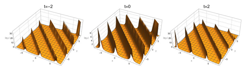
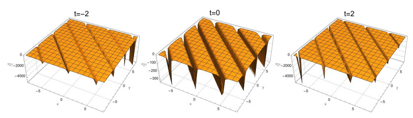
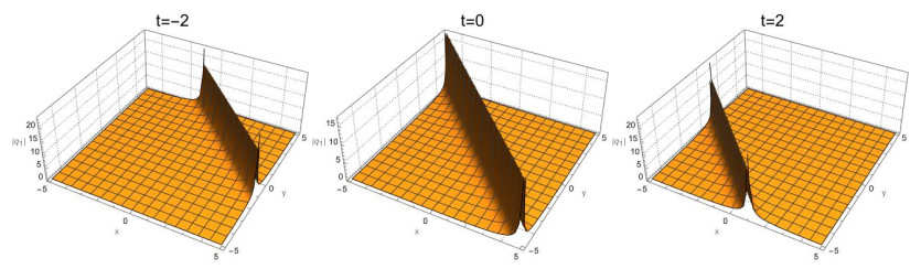
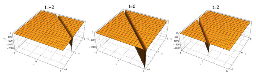
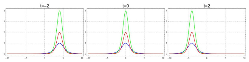
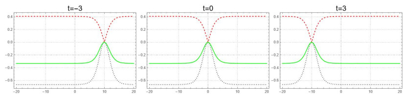
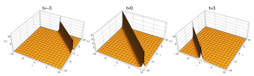
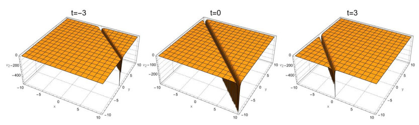
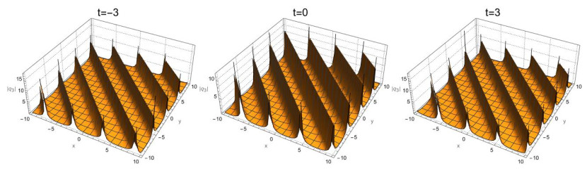
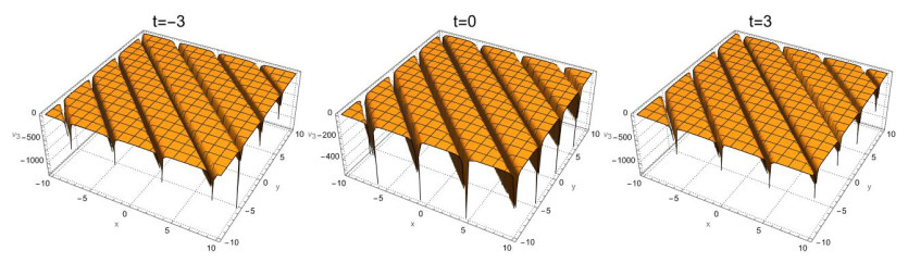
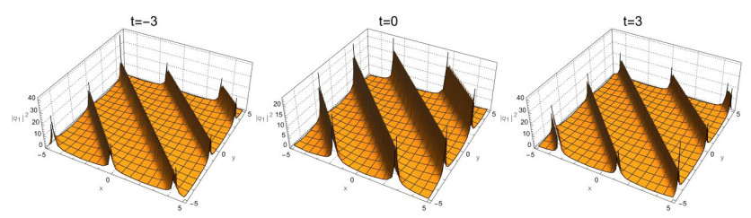
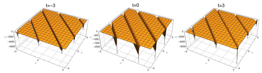
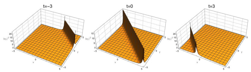
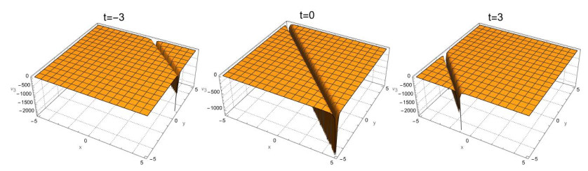
In this paper, the (2+1)-dimensional complex modified Korteweg-de Vries (cmKdV) equations are studied using the sine-cosine method, the tanh-coth method, and the Kudryashov method. As a result, analytical solutions in the form of dark solitons, bright solitons, and periodic wave solutions are obtained. Finally, the dynamic behavior of the solutions is illustrated by choosing the appropriate parameters using 2D and 3D plots. The obtained results show that the proposed methods are straightforward and powerful and can provide more forms of traveling wave solutions, which are expected to be useful for the study of the theory of traveling waves in physics.
- periodic traveling wave,
- bright soliton,
- dark soliton,
- sine-cosine method,
- tanh-coth method,
- Kudryashov method
Citation: Gaukhar Shaikhova, Bayan Kutum, Ratbay Myrzakulov. Periodic traveling wave, bright and dark soliton solutions of the (2+1)-dimensional complex modified Korteweg-de Vries system of equations by using three different methods[J]. AIMS Mathematics, 2022, 7(10): 18948-18970. doi: 10.3934/math.20221043

Related Papers:

Abstract

In this paper, the (2+1)-dimensional complex modified Korteweg-de Vries (cmKdV) equations are studied using the sine-cosine method, the tanh-coth method, and the Kudryashov method. As a result, analytical solutions in the form of dark solitons, bright solitons, and periodic wave solutions are obtained. Finally, the dynamic behavior of the solutions is illustrated by choosing the appropriate parameters using 2D and 3D plots. The obtained results show that the proposed methods are straightforward and powerful and can provide more forms of traveling wave solutions, which are expected to be useful for the study of the theory of traveling waves in physics.

References

[1]	M. J. Ablowitz, P. A. Clarkson, Solitons, Nonlinear Evolution Equations and Inverse Scatetering, Cambridge University Press, Cambridge, UK, 1991. https://doi.org/10.1017/CBO9780511623998
[2]	A. Wazwaz, Partial Differential Equations and Solitary Waves Theory, Springer, Berlin, 2009. https://doi.org/10.1007/978-3-642-00251-9
[3]	J. G. Liu, M. S.Osman, Nonlinear dynamics for different nonautonomous wave structures solutions of a 3D variable-coefficient generalized shallow water wave equation. Chinese J. Phys., 77 (2022), 1618–1624. https://doi.org/10.1016/j.cjph.2021.10.026 doi: 10.1016/j.cjph.2021.10.026
[4]	J. G. Liu, H. Zhao. Multiple rogue wave solutions for the generalized (2+1)-dimensional Camassa–Holm–Kadomtsev–Petviashvili equation, Chinese J. Phys., 77 (2022), 985–991. https://doi.org/10.1016/j.cjph.2021.10.010 doi: 10.1016/j.cjph.2021.10.010
[5]	W. H. Zhu, F. Y. Liu, J. G. Liu, Nonlinear dynamics for different nonautonomous wave structures solutions of a (4+1)-dimensional variable-coefficient Kadomtsev–Petviashvili equation in fluid mechanics, Nonlinear Dynam., 108 (2022), 4171–4180. https://doi.org/10.1515/phys-2022-0050 doi: 10.1515/phys-2022-0050
[6]	D. J. Korteweg, G. de Vries, On the change of form of long waves advancing in a rectangular canal, and on a new type of long stationary waves, Philosophical Magazine Series 5, 39 (1895), 422–443. https://doi.org/10.1080/14786449508620739 doi: 10.1080/14786449508620739
[7]	R. M. Miura, C. S. Gardner, M. S. Kruskal, Korteweg-de Vries equation and generalizations. Ⅱ, Existence of conservation laws and constants of motion, J. Math. Phys., 9 (1968), 1204–1209. https://doi.org/10.1063/1.1664701 doi: 10.1063/1.1664701
[8]	R. Hirota, Exact solution of the modified Korteweg-de Vries equation for multiple collisions of solitons, J. Phys. Soc. Jpn., 22 (1972), 1456–1458. https://doi.org/10.1143/JPSJ.33.1456 doi: 10.1143/JPSJ.33.1456
[9]	M. Wadati, The exact solution of the modified Korteweg–de Vries equation, J. Phys. Soc. Jpn., 32 (1972), 1681–1681. https://doi.org/10.1143/JPSJ.32.1681. doi: 10.1143/JPSJ.32.1681
[10]	R. Hirota, Exact solution of the modified Korteweg–de Vries equation for multiple collisions of solitons, J. Phys. Soc. Jpn., 33 (1972), 1456–1458. https://doi.org/10.1143/JPSJ.33.1456 doi: 10.1143/JPSJ.33.1456
[11]	W. Liu, Y. S. Zhang, J. S. He, Dynamics of the smooth positons of the complex modified KdV equation, Wave. Random Complex, 28 (2018), 203–214. https://doi.org/10.1080/17455030.2017.1335916 doi: 10.1080/17455030.2017.1335916
[12]	A. M. Wazwaz, The tanh and the sine-cosine methods for the complex modified KdV and the generalized KdV equations, Comput. Math. Appl., 49 (2005), 1101–1112. https://doi.org/10.1016/j.camwa.2004.08.013 doi: 10.1016/j.camwa.2004.08.013
[13]	J. He, L. Wang, L. Li, K. Porseizian, R. Erdely, Few-cycle optical rogue waves: Compex modified Korteweg-de Vries equation, Phys. Rev. E, 89 (2014), 062917. https://doi.org/10.1103/PhysRevE.89.062917 doi: 10.1103/PhysRevE.89.062917
[14]	S. C. Anco, T. Ngatat, M. Willoughby, Interaction properties of complex modified Kortewe-de Vries (mKdV) solitons, Physica D, 240 (2011), 1378–1394. https://doi.org/10.1016/j.physd.2011.06.003 doi: 10.1016/j.physd.2011.06.003
[15]	J. S. He, L. H. Wang, L. J. Li, K. Porsezian, R. Erdelyi, Few-cycle optical rogue waves: Complex modified Korteweg-de Vries equation, Phys. Rev. E, 89 (2014), 062917. https://doi.org/10.1103/PhysRevE.89.062917 doi: 10.1103/PhysRevE.89.062917
[16]	T. X. Xu, Z. J. Qiao, Y. Li, Darboux transformation and shock solitons for complex mKdV equation, Pacific J. Appl. Math., 3 (2011), 137.
[17]	Y. Kivshar, G. P. Agrawal, Optical Solitons: From Fibers to Photonic Crystals, Boston: Academic, 2003.
[18]	K. J. Wang, Traveling wave solutions of the Gardner equation in dusty plasmas, Results Phys., 33 (2022), 105207. https://doi.org/10.1016/j.rinp.2022.105207 doi: 10.1016/j.rinp.2022.105207
[19]	K. J. Wang, Abundant exact soliton solutions to the Fokas system, Optik, 249 (2022), 168265. https://doi.org/10.1016/j.ijleo.2021.168265 doi: 10.1016/j.ijleo.2021.168265
[20]	V. Matveev, M. A. Salle, Darboux Transformations and Solitons, Springer-Verlag, Berlin, Germany, 1991. http://dx.doi.org/10.1007/978-3-662-00922-2
[21]	K. Yesmakhanova, G. Bekova, G. Shaikhova, R. Myrzakulov, Soliton solutions of the (2+1)-dimensional complex modified Korteweg-de Vries and Maxwell-Bloch equations, J. Phys.: Conference Series, 738 (2016), 012018. https://doi.org/10.1088/1742-6596/738/1/012018 doi: 10.1088/1742-6596/738/1/012018
[22]	W. H. Zhu, J. G. Liu, Stripe solitons and lump solutions to a generalized (3+1)-dimensional B-type Kadomtsev-Petviashvili equation with variable coefficients in fluid dynamics, J. Math. Anal. Appl., 502 (2021), 125198. https://doi.org/10.1016/j.jmaa.2021.125198 doi: 10.1016/j.jmaa.2021.125198
[23]	J. G. Liu, W. H. Zhu, Multiple rogue wave, breather wave and interaction solutions of a generalized (3 + 1)-dimensional variable-coefficient nonlinear wave equation, Nonlinear Dynam., 103 (2021), 1841–1850. https://doi.org/10.1007/s11071-020-06186-1 doi: 10.1007/s11071-020-06186-1
[24]	J. G. Liu, W. H. Zhu, M. S. Osman, W. X. Ma, An explicit plethora of different classes of interactive lump solutions for an extension form of 3D-Jimbo–Miwa model, Eur. Phys. J. Plus, 135 (2020), 412. https://doi.org/10.1140/epjp/s13360-020-00405-9 doi: 10.1140/epjp/s13360-020-00405-9
[25]	Y. Tian, J. G. Liu, Study on dynamical behavior of multiple lump solutions and interaction between solitons and lump wave, Nonlinear Dynam., 104 (2021), 1507–1517. https://doi.org/10.1007/s11071-021-06322-5 doi: 10.1007/s11071-021-06322-5
[26]	J. G. Liu, W. H. Zhu, Y. He, Variable-coefficient symbolic computation approach for finding multiple rogue wave solutions of nonlinear system with variable coefficients, Zeitschrift für angewandte Mathematik und Physik, 72 (2021), 154. https://doi.org/10.1007/s00033-021-01584-w doi: 10.1007/s00033-021-01584-w
[27]	K. J. Wang, J. Si, Investigation into the Explicit Solutions of the Integrable (2+1)-Dimensional Maccari System via the Variational Approach, Axioms, 11 (2022), 234. https://doi.org/10.3390/axioms11050234 doi: 10.3390/axioms11050234
[28]	K. J. Wang, G. D. Wang, Variational theory and new abundant solutions to the (1+2)-dimensional chiral nonlinear Schrödinger equation in optics, Phys. Lett. A, 412 (2021), 127588. https://doi.org/10.1016/j.physleta.2021.127588 doi: 10.1016/j.physleta.2021.127588
[29]	A. M. Wazwaz, The sine-cosine method for obtaining solutions with compact and noncompact structures, Appl. Math. Comput., 159 (2004), 559–576. https://doi.org/10.1016/j.amc.2003.08.136 doi: 10.1016/j.amc.2003.08.136
[30]	E. Yusufoglu, A. Bekir, Solitons and periodic solutions of coupled nonlinear evolution equations by using Sine-Cosine method. Int. J. Comput. Math., 83 (2006), 915–924. https://doi.org/10.1080/00207160601138756 doi: 10.1080/00207160601138756
[31]	S. Albosaily, W. W. Mohammed, M. A. Aiyashi, M. A. Abdelrahman, Exact solutions of the (2 + 1)-dimensional stochastic chiral nonlinear Schrödinger equation, Mathematics, 8 (2020), 1889(1–12). https://doi.org/10.3390/sym12111874 doi: 10.3390/sym12111874
[32]	W. Malfliet, Solitary wave solutions of nonlinear wave equations, Am. J. Phys., 60 (1992), 650–654. https://doi.org/10.1119/1.17120 doi: 10.1119/1.17120
[33]	W. Malfliet, W. Hereman, The Tanh method: Ⅱ Perturbation technique for conservative systems, Phys. Scripta, 54 (1996), 569–575. https://doi.org/10.1088/0031-8949/54/6/004 doi: 10.1088/0031-8949/54/6/004
[34]	W. Malfliet, The tanh method: A tool for solving certain classes of nonlinear evolution and wave equations, J. Comput. Appl. Math., 164–165 (2004), 529–541. https://doi.org/10.1016/S0377-0427(03)00645-9 doi: 10.1016/S0377-0427(03)00645-9
[35]	N. B. Ivanov, J. Ummethum, J. Schnack, Phase diagram of the alternating-spin Heisenberg chain with extra isotropic three-body exchange interactions, Eur. Phys. J. B, 87 (2014), 1–13. https://doi.org/10.1140/epjb/e2014-50423-7 doi: 10.1140/epjb/e2014-50423-7
[36]	R. Myrzakulov, G. K. Mamyrbekova, G. N. Nugmanova, K. R. Yesmakhanova, M. Lakshmanan, Integrable motion of curves in self-consistent potentials: Relation to spin systems and soliton equations, Phys. Lett. A, 378 (2014), 2118–2123. https://doi.org/10.1016/j.physleta.2014.05.010 doi: 10.1016/j.physleta.2014.05.010
[37]	K. Yesmakhanova, G. Nugmanova, G. Shaikhova, G. Bekova, R. Myrzakulov, Coupled dispersionless and generalized Heisenberg ferromagnet equations with self-consistent sources: Geometry and equivalence, Int. J. Geom. Methods M., 17 (2020), 2050104. https://doi.org/10.1142/S0219887820501042 doi: 10.1142/S0219887820501042
[38]	K. Porsezian, M. Daniel, M. Lakshmanan, On the integrability aspects of the one-dimensional classical continuum isotropic Heisenberg spin chain, J. Math. Phys., 33 (1992), 1807–1816. https://doi.org/10.1063/1.529658 doi: 10.1063/1.529658
[39]	R. Myrzakulov, G. K. Mamyrbekova, G. N. Nugmanova, M. Lakshmanan, Integrable (2+1)-dimensional spin models with self-consistent potentials, Symmetry, 7 (2015), 1352–1375. https://doi.org/10.3390/sym7031352 doi: 10.3390/sym7031352
[40]	K. Yesmakhanova, G. Shaikhova, G. Bekova, R. Myrzakulov, Darboux transformation and soliton solution for the (2+1)-dimensional complex modified Korteweg-de Vries equations, J. Phys. Conf. Ser., 936 (2017), 012045. https://doi.org/10.1088/1742-6596/936/1/012045 doi: 10.1088/1742-6596/936/1/012045
[41]	F. Yuan, X. Zhu, Y. Wang, Deformed solitons of a typical set of (2+1)–dimensional complex modified Korteweg–de Vries equations, Int. J. Appl. Math. Comput. Sci., 30 (2020), 337–350. https://doi.org/10.34768/amcs-2020-0026 doi: 10.34768/amcs-2020-0026
[42]	F. Yuan, Y. Jiang, Periodic solutions of the (2 + 1)-dimensional complex modifed Korteweg-de Vries equation, Modern Phys. Lett. B, 34 (2020), 2050202(1-10). https://doi.org/10.1142/S0217984920502024 doi: 10.1142/S0217984920502024
[43]	F. Yuan, The order-n breather and degenerate breather solutions of the (2+1)-dimensional cmKdV equations, Int. J. Modern Phys. B, 35 (2021), 2150053. https://doi.org/10.1142/S021797922150053 doi: 10.1142/S021797922150053
[44]	G. N. Shaikhova, N. Serikbayev, K. Yesmakhanova, R. Myrzakulov, Nonlocal complex modified Korteweg-de Vries equations: Reductions and exact solutions, Proceedings of the Twenty-First International Conference on Geometry, Integrability and Quantization, (2020), 265–271. https://doi.org/10.7546/giq-21-2020-265-271
[45]	A. M. Wazwaz, The Camassa–Holm–KP equations with compact and noncompact travelling wave solutions, Appl. Math. Comput., 170 (2005), 347–360. https://doi.org/10.1016/j.amc.2004.12.002 doi: 10.1016/j.amc.2004.12.002
[46]	A. M. Wazwaz, Solitons and periodic solutions for the fifth-order KdV equation, Appl. Math. Lett., 19 (2006), 1162–1167. https://doi.org/10.1016/j.aml.2005.07.014 doi: 10.1016/j.aml.2005.07.014
[47]	G. N. Shaikhova, B. B. Kutum, Traveling wave solutions of two-dimensional nonlinear Schrodinger equation via sine-cosine method, Eurasian Phys. Technical J., 17 (2020), 169–174. http://rep.ksu.kz/xmlui/handle/data/10854
[48]	J. Javadvahidi, S. M. Zekavatmanda, H. Rezazadeh, M. Mehmet, A. Akinlar, Y. Ch. Chugh, New solitary wave solutions to the coupled Maccari's system, Res. Phys., 21 (2021), 103801. https://doi.org/10.1016/j.rinp.2020.103801 doi: 10.1016/j.rinp.2020.103801
[49]	A. M. Wazwaz, The extended tanh method for new solitons solutions for many forms of the fifth-order KdV equations, Appl. Math. Comput., 184 (2007), 1002–1014. https://doi.org/10.1016/j.amc.2006.07.002 doi: 10.1016/j.amc.2006.07.002
[50]	K. J. Wang, Abundant analytical solutions to the new coupled Konno-Oono equation arising in magnetic field, Res. Phys., 31 (2021), 104931. https://doi.org/10.1016/j.rinp.2021.104931 doi: 10.1016/j.rinp.2021.104931
[51]	K. J. Wang, G. D. Wang, Exact traveling wave solutions for the system of the ion sound and Langmuir waves by using three effective methods, Res. Phys., 35 (2022), 105390. https://doi.org/10.1016/j.rinp.2022.105390 doi: 10.1016/j.rinp.2022.105390
[52]	C. Burdik, G. Shaikhova, B. Rakhimzhanov, Soliton solutions and travelling wave solutions for the two-dimensional generalized nonlinear Schrodinger equations, Eur. Phys. J. Plus., 136 (2021), 1095(1–17). https://doi.org/10.1140/epjp/s13360-021-02092-6 doi: 10.1140/epjp/s13360-021-02092-6
[53]	N. A. Kudryashov, Exact soliton solutions of the generalized evolution equation of wave dynamics, J. Appl. Math. Mech., 52 (1988), 361–365. https://doi.org/10.1016/0021-8928(88)90090-1 doi: 10.1016/0021-8928(88)90090-1
[54]	N. A. Kudryashov, Exact solutions of the generalized Kuramoto-Sivashinsky equation, Phys. Lett. A., 147 (1990), 287–291. https://doi.org/10.1016/0375-9601(90)90449-X doi: 10.1016/0375-9601(90)90449-X
[55]	N. A. Kudryashov, On types of nonlinear nonintegrable equations with exact solutions, Phys. Lett. A., 155 (1991), 269–275. https://doi.org10.1016/0375-9601(91)90481-M
[56]	N. A. Kudryashov, Simpliest equation method to look for exact solutions of nonlinear differential equations, Chaos, Soliton. Fract., 24 (2005), 1217–1231. https://doi.org/10.1016/j.chaos.2004.09.109 doi: 10.1016/j.chaos.2004.09.109

Reader Comments

Your name:*

Email:*
© 2022 the Author(s), licensee AIMS Press. This is an open access article distributed under the terms of the Creative Commons Attribution License (http://creativecommons.org/licenses/by/4.0)