Contraction of variational principle and optical soliton solutions for two models of nonlinear Schrödinger equation with polynomial law nonlinearity

Aly R. Seadawy; Bayan Alsaedi; Aly R. Seadawy; Bayan Alsaedi

doi:10.3934/math.2024309

AIMS Mathematics

2024, Volume 9, Issue 3: 6336-6367. doi: 10.3934/math.2024309

Previous Article Next Article

Research article Special Issues

Contraction of variational principle and optical soliton solutions for two models of nonlinear Schrödinger equation with polynomial law nonlinearity

Aly R. Seadawy ^,,
Bayan Alsaedi

Department of Mathematics, Faculty of Science, Taibah University, Al-Madinah Al-Munawarah, Saudi Arabia

Received: 28 November 2023 Revised: 15 January 2024 Accepted: 19 January 2024 Published: 04 February 2024
MSC : 35B10, 35C07, 35C08, 35Q35

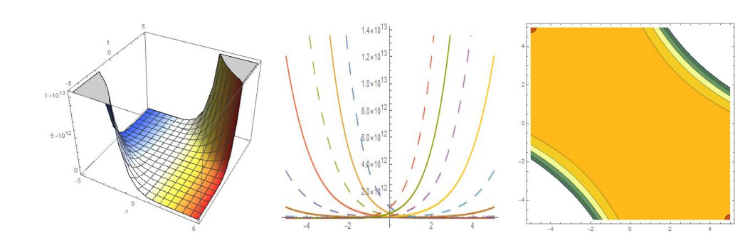
Our study analyzes the two models of the nonlinear Schrödinger equation (NLSE) with polynomial law nonlinearity by powerful and comprehensible techniques, such as the variational principle method and the amplitude ansatz method. We will derive the functional integral and the Lagrangian of these equations, which illustrate the system's dynamic. The solutions of these models will be extracted by selecting the trial ansatz functions based on the Jost linear functions, which are continuous at all intervals. We start with the Jost function that has been approximated by a piecewise linear function with a single nontrivial variational parameter in three cases from a region of a rectangular box, then use this trial function to obtain the functional integral and the Lagrangian of the system without any loss. After that, we approximate this trial function by piecewise linear ansatz function in two cases of the two-box potential, then approximate it by quadratic polynomials with two free parameters rather than a piecewise linear ansatz function, and finally, will be approximated by the tanh function. Also, we utilize the amplitude ansatz method to extract the new solitary wave solutions of the proposed equations that contain bright soliton, dark soliton, bright-dark solitary wave solutions, rational dark-bright solutions, and periodic solitary wave solutions. Furthermore, conditions for the stability of the solutions will be submitted. These answers are crucial in applied science and engineering and will be introduced through various graphs such as 2D, 3D, and contour plots.

Keywords:

Citation: Aly R. Seadawy, Bayan Alsaedi. Contraction of variational principle and optical soliton solutions for two models of nonlinear Schrödinger equation with polynomial law nonlinearity[J]. AIMS Mathematics, 2024, 9(3): 6336-6367. doi: 10.3934/math.2024309

Related Papers:

[1]	Islam Samir, Hamdy M. Ahmed, Wafaa Rabie, W. Abbas, Ola Mostafa . Construction optical solitons of generalized nonlinear Schrödinger equation with quintuple power-law nonlinearity using Exp-function, projective Riccati, and new generalized methods. AIMS Mathematics, 2025, 10(2): 3392-3407. doi: 10.3934/math.2025157
[2]	Elsayed M. E. Zayed, Mona El-Shater, Khaled A. E. Alurrfi, Ahmed H. Arnous, Nehad Ali Shah, Jae Dong Chung . Dispersive optical soliton solutions with the concatenation model incorporating quintic order dispersion using three distinct schemes. AIMS Mathematics, 2024, 9(4): 8961-8980. doi: 10.3934/math.2024437
[3]	Yazid Alhojilan, Islam Samir . Investigating stochastic solutions for fourth order dispersive NLSE with quantic nonlinearity. AIMS Mathematics, 2023, 8(7): 15201-15213. doi: 10.3934/math.2023776
[4]	Dumitru Baleanu, Kamyar Hosseini, Soheil Salahshour, Khadijeh Sadri, Mohammad Mirzazadeh, Choonkil Park, Ali Ahmadian . The (2+1)-dimensional hyperbolic nonlinear Schrödinger equation and its optical solitons. AIMS Mathematics, 2021, 6(9): 9568-9581. doi: 10.3934/math.2021556
[5]	Jinfang Li, Chunjiang Wang, Li Zhang, Jian Zhang . Multi-solitons in the model of an inhomogeneous optical fiber. AIMS Mathematics, 2024, 9(12): 35645-35654. doi: 10.3934/math.20241691
[6]	Ninghe Yang . Exact wave patterns and chaotic dynamical behaviors of the extended (3+1)-dimensional NLSE. AIMS Mathematics, 2024, 9(11): 31274-31294. doi: 10.3934/math.20241508
[7]	Abeer S. Khalifa, Hamdy M. Ahmed, Niveen M. Badra, Wafaa B. Rabie, Farah M. Al-Askar, Wael W. Mohammed . New soliton wave structure and modulation instability analysis for nonlinear Schrödinger equation with cubic, quintic, septic, and nonic nonlinearities. AIMS Mathematics, 2024, 9(9): 26166-26181. doi: 10.3934/math.20241278
[8]	Nafissa T. Trouba, Huiying Xu, Mohamed E. M. Alngar, Reham M. A. Shohib, Haitham A. Mahmoud, Xinzhong Zhu . Soliton solutions and stability analysis of the stochastic nonlinear reaction-diffusion equation with multiplicative white noise in soliton dynamics and optical physics. AIMS Mathematics, 2025, 10(1): 1859-1881. doi: 10.3934/math.2025086
[9]	Abdulah A. Alghamdi . Analytical discovery of dark soliton lattices in (2+1)-dimensional generalized fractional Kundu-Mukherjee-Naskar equation. AIMS Mathematics, 2024, 9(8): 23100-23127. doi: 10.3934/math.20241123
[10]	Yousef F. Alharbi, E. K. El-Shewy, Mahmoud A. E. Abdelrahman . New and effective solitary applications in Schrödinger equation via Brownian motion process with physical coefficients of fiber optics. AIMS Mathematics, 2023, 8(2): 4126-4140. doi: 10.3934/math.2023205

Abstract

1. Introduction

The nonlinear Schrödinger equations (NLSEs) are extensively used to describe numerous crucial phenomena and dynamic processes in various fields such as fluid dynamics, plasma, chemistry, biology, optical fibers^[1,2,3,4], nuclear physics, stochastic mechanics, biomolecule dynamics, dynamics of accelerators, and Bose-Einstein condensates ^{[5,6,7,8,9,10]}. The last few decades have seen significant advancements in the field of nonlinear optics ^[11,12,13]. These equations also appear in other forms of nonlinearities, such as cubic-quintic (CQ), cubic-quintic-septic (CQS), power-law, logarithmic nonlinearities, and various other forms. There is a growing interest in studying soliton pulses that can propagate without changing their shape in optical fibers ^[14,15].

Therefore, obtaining the exact soliton solutions of these NLSEs can help us to understand these phenomena better. In recent years, several effective approaches have been developed to construct accurate solutions of these equations. For example, the simple equation method ^[16], Kudryashov's method ^[17], the Jacobi elliptic function method ^[18], the inverse scattering method ^[19], the extended trial function method ^[20], the tanh method ^[21], the F-expansion method ^[22], generalized extended tanh-function method, the sine–cosine method ^[23], the generalized Riccati equation method ^[24], the new $\phi^6$ -model expansion method ^[25], Hirota bilinear method ^[26], the exp-function method ^[27], the Darboux transformation ^[28], the auxiliary equation method ^[29], the Binary Bell polynomials ^[30], the extended hyperbolic function method ^[31], the homogeneous balance Method ^[32], the $(\frac{G'}{G})$ -expansion method ^[33,34], the exponential rational function method ^[35], the Bäcklund transformation ^[36], the homotopy perturbation method ^[37], the modified Kudryashov method, the sine-Gordon expansion approach ^[38], the Riccati-Bernoulli sub-ODE method ^[39], the modified extended direct algebraic method ^[40], the truncated Painlevé expansion method ^[41], the $(G'/G, 1/G)$ -expansion method ^[42], the tan $(\phi/2)$ -expansion method ^[43,44], the soliton ansatz method ^[45,46], and so on.

Researches have been conducted on the study of NLSEs with the polynomial law of nonlinearity. For instance, Seadawy et al. ^[47] established soliton solutions using the extended simplest equation method, and they also described this model ^[48], which includes the conservation principles for optical soliton (OS) with polynomial and triple power law nonlinearities, while Aziz et al. ^[49] discovered chirped soliton solutions by utilizing Jacobi elliptic functions. Furthermore, this model was discussed by Dieu-donne et al. ^[50], who examined the optical soliton (OS) solutions with two types of nonlinearities, which are triple power and polynomial laws. Sugati et al.^[51] also examined this model, obtaining the traveling pulse solutions to the NLSE when it is treated with both spatio-temporal dispersion (STD) and group velocity dispersion (GVD).

In this paper, our aim is to investigate soliton solutions for two models of the NLSE that carry the polynomial law of nonlinearity (cubic-quintic-septic). We will use the variational principle based on finding Lagrangian, which we will then apply it with different trial functions that have one or two nontrivial variational parameters. Furthermore, we will employ another technique called the amplitude ansatz method to extract new solitary wave solutions.

The paper is categorized as follows. In Section 2, we discuss model-I of NLSE with polynomial law nonlinearity in terms of formulation of the variational principle and finding solitary wave solutions. In Section 3, we apply the same steps on model-II of NLSE with polynomial law nonlinearity. Finally, the work concludes in Section 4.

2. Schrödinger's nonlinear equation with the polynomial nonlinear law model I

2.1. Formulation of the variational principle for the Schrödinger's nonlinear equation with the polynomial nonlinear law

Nonlinear Schrödinger equation (NLSE) with the polynomial nonlinear law is ^[47]:

$\begin{equation} i\Gamma_t+a\Gamma_{xx}+b_1\Gamma|\Gamma|^2+b_2\Gamma|\Gamma|^4+b_3\Gamma|\Gamma|^6 = 0. \end{equation}$

(2.1)

Such that $\Gamma$ is a complex function on the form: $\Gamma(x, t) = \Theta(x, t)+i\Psi(x, t)$ . Since $\Theta$ and $\Psi$ are real functions of $x$ and $t$ , furthermore $|\Gamma|^2 = (\Theta+i\Psi)(\Theta-i\Psi)$ . Using the variational approach, we will search for solutions to NLSE with the polynomial nonlinear law. As a result, we derive $\Gamma$ with respect to $x$ and $t$ to investigate the existence of a Lagrangian and the invariant variational principle for this equation, which are expressed in the following way:

Let $M$ and $N$ are functionals in $\Theta$ and $\Psi$ :

$\begin{equation} \begin{aligned} M(\Theta, \Psi) = &\frac{\partial \Theta}{\partial t}+a \frac{\partial^2\Psi}{\partial x^2}+b_1\Psi\Theta^2+b_1\Psi^3+b_2\Psi\Theta^4+2b_2\Theta^2\Psi^3+b_2\Psi^5+b_3\Psi\Theta^6\\&+3b_3\Theta^4\Psi^3+3b_3\Theta^2\Psi^5+b_3\Psi^7, \end{aligned} \end{equation}$

(2.2)

$\begin{equation} \begin{aligned} N(\Theta, \Psi) = &-\frac{\partial \Psi}{\partial t}+a \frac{\partial^2\Theta}{\partial x^2}+b_1\Theta^3+b_1\Theta\Psi^2+b_2\Theta^5+2b_2\Psi^2\Theta^3+b_2\Theta\Psi^4+b_3\Theta^7\\&+3b_3\Psi^2\Theta^5+3b_3\Theta^3\Psi^4+b_3\Theta\Psi^6. \end{aligned} \end{equation}$

(2.3)

Put $\Theta = \lambda\Theta$ and $\Psi = \lambda\Psi$ ,

$\begin{aligned} \int_0^1M(\lambda\Theta, \lambda\Psi)\, d\lambda = &\frac{1}{2}\frac{\partial \Theta}{\partial t}+\frac{1}{2}a \frac{\partial^2\Psi}{\partial x^2}+\frac{1}{4}b_1\Psi\Theta^2+\frac{1}{4}b_1\Psi^3+\frac{1}{6}b_2\Psi\Theta^4+\frac{1}{3}b_2\Theta^2\Psi^3\\&+\frac{1}{6}b_2\Psi^5+\frac{1}{8}b_3\Psi\Theta^6+\frac{3}{8}b_3\Theta^4\Psi^3+\frac{3}{8}b_3\Theta^2\Psi^5+\frac{1}{8}b_3\Psi^7, \end{aligned}$

$\begin{aligned} \int_0^1N(\lambda \Theta, \lambda\Psi)\, d\lambda = &-\frac{1}{2}\frac{\partial \Psi}{\partial t}+\frac{1}{2}a\frac{\partial^2\Theta}{\partial x^2}+\frac{1}{4}b_1\Theta^3+\frac{1}{4}b_1\Theta\Psi^2+\frac{1}{6}b_2\Theta^5+\frac{1}{3}b_2\Psi^2\Theta^3\\&+\frac{1}{6}b_2\Theta\Psi^4+\frac{1}{8}b_3\Theta^7+\frac{3}{8}b_3\Psi^2\Theta^5+\frac{3}{8}b_3\Theta^3\Psi^4+\frac{1}{8}b_3\Theta\Psi^6. \end{aligned}$

The consistency conditions are expressed as follows ^[52,53], where $\Theta_x$ , $\Psi_x$ , $\Theta_t$ and $\Psi_t$ stand for the partial derivatives of $\Theta$ and $\Psi$ with respect to variables $x$ and $t$ . If the system of Eqs (2.2) and (2.3) satisfies the the previously mentioned conditions, then a functional integral $J(\Theta, \Psi)$ can be written down using the formula given by Tonti ^[53]:

$\begin{aligned} J(\Theta, \Psi) = &\int_\omega\Big[\frac{1}{4}b_1\Theta^4+\frac{1}{6}b_2\Theta^6+\frac{1}{8}b_3\Theta^8+\frac{1}{2}b_1\Theta^2\Psi^2+\frac{1}{2}b_2\Theta^4\Psi^2+\frac{1}{2}b_3\Theta^6\Psi^2\\&+\frac{1}{4}b_1\Psi^4+\frac{1}{2}b_2\Theta^2\Psi^4+\frac{3}{4}b_3\Theta^4\Psi^4+\frac{1}{6}b_2\Psi^6+\frac{1}{2}b_3\Theta^2\Psi^6+\frac{1}{8}b_3\Psi^8\\&+\frac{1}{2}\Psi\Theta_t-\frac{1}{2}\Theta\Psi_t+\frac{1}{2}a\Theta\Theta_{xx}+\frac{1}{2}a\Psi\Psi_{xx}\Big] \;d\omega, \end{aligned}$

where $d\omega = dxdt$ .

The terms $\Theta\Theta_{xx}$ and $\Psi\Psi_{xx}$ solve integration by parts and choosing the boundary on $\Theta_x$ and $\Psi_x$ to be such that the boundary terms vanish, we get

$\begin{equation} \begin{aligned} J(\Theta, \Psi) = &\int_\omega \Big[ \frac{1}{4}b_1\Theta^4+\frac{1}{6}b_2\Theta^6+\frac{1}{8}b_3\Theta^8+\frac{1}{2}b_1\Theta^2\Psi^2+\frac{1}{2}b_2\Theta^4\Psi^2+\frac{1}{2}b_3\Theta^6\Psi^2\\&+\frac{1}{4}b_1\Psi^4+\frac{1}{2}b_2\Theta^2\Psi^4+\frac{3}{4}b_3\Theta^4\Psi^4+\frac{1}{6}b_2\Psi^6+\frac{1}{2}b_3\Theta^2\Psi^6+\frac{1}{8}b_3\Psi^8\\&+\frac{1}{2}\Psi\Theta_t-\frac{1}{2}\Theta\Psi_t-\frac{1}{2}a\Theta_x^2-\frac{1}{2}a\Psi_x^2 \Big] \;d\omega, \end{aligned} \end{equation}$

(2.4)

where $d\omega = dxdt$ .

We obtain the Lagrangian $L$ as

$\begin{equation} \begin{aligned} L(\Theta, \Psi) = &\frac{1}{4}b_1\Theta^4+\frac{1}{6}b_2\Theta^6+\frac{1}{8}b_3\Theta^8+\frac{1}{2}b_1\Theta^2\Psi^2+\frac{1}{2}b_2\Theta^4\Psi^2+\frac{1}{2}b_3\Theta^6\Psi^2\\&+\frac{1}{4}b_1\Psi^4+\frac{1}{2}b_2\Theta^2\Psi^4+\frac{3}{4}b_3\Theta^4\Psi^4+\frac{1}{6}b_2\Psi^6+\frac{1}{2}b_3\Theta^2\Psi^6+\frac{1}{8}b_3\Psi^8\\&+\frac{1}{2}\Psi\Theta_t-\frac{1}{2}\Theta\Psi_t-\frac{1}{2}a\Theta_x^2-\frac{1}{2}a\Psi_x^2. \end{aligned} \end{equation}$

(2.5)

We find the value of $L$ in the Euler-Lagrange equations to validate our interpretations:

$\frac{\partial L}{\partial \Theta}-\frac{\partial}{\partial t}\left(\frac{\partial L}{\partial \Theta_t}\right)-\frac{\partial}{\partial x}\left(\frac{\partial L}{\partial \Theta_{x}} \right) = 0,$

$\frac{\partial L}{\partial \Psi}-\frac{\partial}{\partial t}\left(\frac{\partial L}{\partial \Psi_t}\right)-\frac{\partial}{\partial x}\left(\frac{\partial L}{\partial \Psi_{x}} \right) = 0.$

The resulting derivatives give us the system of Eqs (2.2) and (2.3).

2.1.1. The rectangular box

We demonstrate the simplest example of the application of this technique, by taking the box-shaped initial pulse and an ansatz based on linear Jost functions in a single nontrivial variational parameter in three cases.

Case 1: We use the following ansatz for $\Theta(x, t)$ and $\Psi(x, t)$ functions:

$\begin{equation} \Theta(x, t) = \begin{cases} 100 \exp (-\mu(t-5)(x-5)), & \text{at} \quad x > 5, \; t > 5, \\ (t+5)(x+5), & \text{at} \quad |x| < 5, \; |t| < 5 , \\ 0, & \text{at} \quad x < -5, \; t < -5, \end{cases} \end{equation}$

(2.6)

$\begin{equation} \Psi(x, t) = \begin{cases} 0, & \text{at} \quad x > 5, \; t > 5, \\ (5-t)(5-x), & \text{at} \quad |x| < 5, \; |t| < 5, \\ 100 \exp(\mu (t+5)(x+5)), & \text{at} \quad x < -5, \; t < -5. \end{cases} \end{equation}$

(2.7)

We found the values of the Lagrangian $L$ from substituting Eqs (2.6) and (2.7) into Eq (2.5) (see Figure 1):

$J(\Theta, \Psi) = \int_{-\infty}^{-5} \int_{-\infty}^{-5} L \; dxdt + \int_{-5}^{5} \int_{-5}^{5} L \; dxdt + \int_{5}^{\infty} \int_{5}^{\infty} L \; dxdt,$

Figure 1. Show an example of the Lagrangian

$L(x, t)$ with Eq (2.5), in the interval

$-5 < x < 5$ and

$-5 < t < 5$ , by choosing the trial functions (2.6) and (2.7) at

$a = 3, \, b_1 = 2, \, b_2 = \frac{1}{2}, \, b_3 = \frac{1}{6}$ .

DownLoad: Full-Size Img PowerPoint

where

$\int_{-\infty}^{-5} \int_{-\infty}^{-5} L \; dxdt = \int_{5}^{\infty} \int_{5}^{\infty} L \; dxdt = 0.$

By using Mathematica program we get the value of $J(\Theta, \Psi)$ at interval $-5 < x < 5, \, -5 < t < 5$ as

$\begin{equation} \begin{aligned} J(\Theta, \Psi) = & -\frac{10000 a}{3}+\frac{1850000000 b_1}{9}+\frac{304000000000000 b_2}{441} \\& +\frac{1760000000000000000 b_3}{567}+\frac{25000}{3}. \end{aligned} \end{equation}$

(2.8)

Case 2: Assume $\Theta(x, t)$ and $\Psi(x, t)$ for the Jost function as the following:

$\begin{equation} \Theta(x, t) = \begin{cases} 20 \exp (-\mu(t-5)(x-5)), & \text{at} \quad x > 5, \; t > 5, \\ t+x+10, & \text{at} \quad |x| < 5, \; |t| < 5, \\ 0, & \text{at} \quad x < -5, \; t < -5, \end{cases} \end{equation}$

(2.9)

$\begin{equation} \Psi(x, t) = \begin{cases} 0, & \text{at} \quad x > 5, \; t > 5, \\ 10-t-x, & \text{at} \quad |x| < 5, \; |t| < 5, \\ 20 \exp(\mu (t+5)(x+5)), & \text{at} \quad x < -5, \; t < -5. \end{cases} \end{equation}$

(2.10)

We found the values of the Lagrangian $L$ from substituting by Eqs (2.9) and (2.10) into Eq (2.5), then we get

$\begin{equation} J(\Theta, \Psi) = \frac{100}{63} \left(-63 a+882000 b_1+145800000 b_2+28120000000 b_3+630\right). \end{equation}$

(2.11)

Case 3:

$\begin{equation} \Theta(x, t) = \begin{cases} \frac{1}{2}(\exp(6\pi-t-x)-\exp(-2\pi-t-x)), & \text{at} \quad x > \pi, \; t > \pi, \\ \sinh(t+x+2\pi), & \text{at} \quad |x| < \pi, \; |t| < \pi, \\ 0, & \text{at} \quad x < -\pi, \; t < -\pi, \end{cases} \end{equation}$

(2.12)

$\begin{equation} \psi(x, t) = \begin{cases} 0, & \text{at} \quad x > \pi, \; t > \pi, \\ \sinh(2\pi-t-x), & \text{at} \quad |x| < \pi, \; |t| < \pi, \\ \frac{1}{2}(\exp(6\pi+t+x)-\exp(-2\pi+t+x)), & \text{at} \quad x < -\pi, \; t < -\pi. \end{cases} \end{equation}$

(2.13)

We found the values of the Lagrangian $L$ from substituting by Eqs (2.12) and (2.13) into Eq (2.5), then we have

$\begin{equation} \begin{aligned} J(\Theta, \Psi) = & -1.02783\times 10^{10} a+2.64108\times 10^{19} b_1+1.60864\times 10^{29} b_2 \\& +1.39506\times 10^{39} b_3+2.83012\times 10^6. \end{aligned} \end{equation}$

(2.14)

2.1.2. The two-box potential

Case 1: We try the following Jost functions:

$\begin{equation} \Theta(x, t) = \left\{ \begin{array}{lll} \frac{1}{2}\Big(\exp(\pi^2(3+2 \alpha +\alpha^2)-\pi t -\pi x) \\ -\exp(\pi^2(1-2 \alpha -\alpha^2)-\pi t-\pi x)\Big), & \text{at} & x > \pi, \; t > \pi, \\ \sinh((\pi+\alpha t)(\pi+\alpha x)), & \text{at} & 0 < x < \pi, \, 0 < t < \pi, \\ \sinh((t+\pi)(x+\pi)), &\text{at} & -\pi < x < 0, \, -\pi < t < 0 , \\ 0, & \text{at} & x < -\pi, \, t < -\pi, \end{array} \right. \end{equation}$

(2.15)

$\begin{equation} \Psi(x, t) = \left\{ \begin{array}{lll} 0, & \text{at} & x > \pi, \, t > \pi, \\ \sinh((\pi-t)(\pi-x)), & \text{at} & 0 < x < \pi, \, 0 < t < \pi, \\ \sinh((\pi-\alpha t)(\pi-\alpha x)), & \text{at} & -\pi < x < 0, \, -\pi < t < 0, \\ \frac{1}{2}\Big(\exp(\pi^2(3+2 \alpha +\alpha^2)+\pi t+\pi x)\\ -\exp(\pi^2(1-2 \alpha-\alpha^2)+\pi t+\pi x)\Big), & \text{at} & x < -\pi, \; t < -\pi. \end{array} \right. \end{equation}$

(2.16)

This ansatz now contains nontrivial variational parameter $\alpha$ . Substituting Eqs (2.15) and (2.16) into Eq (2.5) (see ), then we obtain the functional integral at $\alpha = -1$ as follows:

$\begin{equation} J(\Theta, \Psi) = -4.43569\times 10^7 a+1.13554\times 10^{14} b_1+6.23167\times 10^{21} b_2+4.89178\times 10^{29} b_3. \end{equation}$

(2.17)

Figure 2. Show an example of the Lagrangian

$L(x, t)$ with Eq (2.5), in the interval

$0 < x < \pi$ and

$0 < t < \pi$ , by choosing the trial functions (2.15) and (2.16) at the parameter

$\alpha = -1$ and

$a = 3, \, b_1 = 2, \, b_2 = \frac{1}{2}, \, b_3 = \frac{1}{6}$ .

DownLoad: Full-Size Img PowerPoint

Also, we can use $\alpha = 2$ , then we get

$\begin{equation*} \begin{aligned} \int_{-\pi}^{0} \int_{-\pi}^{0} L \; dxdt = \int_{0}^{\pi} \int_{0}^{\pi} L \; dxdt = &-4.42653\times 10^{75} a+5.59314\times 10^{148} b_1 +5.89626\times 10^{224} b_2 \\& +8.85443\times 10^{300} b_3-2.66975\times 10^{36}. \end{aligned} \end{equation*}$

The functional integral at $\alpha = 2$ becomes

$\begin{equation} \begin{aligned} J(\Theta, \Psi) = & -1.77562\times 10^{76} a+4.12756\times 10^{150} b_1+4.35525\times 10^{226} b_2 \\& +6.5433\times 10^{302} b_3-5.33949\times 10^{36}. \end{aligned} \end{equation}$

(2.18)

Case 2: We now try the following Jost function:

$\begin{equation} \Theta(x, t) = \left\{ \begin{array}{lll} \frac{1}{2}\Big(\exp(4\pi-t-x+2 \pi \alpha) \\ -\exp(-t-x-2 \pi \alpha)\Big), & \text{at} & x > \pi, \; t > \pi, \\ \sinh(2 \pi+\alpha t+\alpha x), & \text{at} & 0 < x < \pi, \, 0 < t < \pi, \\ \sinh(2\pi+t+x), & \text{at} & -\pi < t < 0, \, -\pi < x < 0, \\ 0, & \text{at} & x < -\pi, \; t < -\pi, \end{array} \right. \end{equation}$

(2.19)

$\begin{equation} \Psi(x, t) = \left\{ \begin{array}{lll} 0, & \text{at} & x > \pi, \; t > \pi, \\ \sinh(2\pi-t-x), & \text{at} & 0 < x < \pi , \; 0 < t < \pi, \\ \sinh(2\pi-\alpha t-\alpha x), & \text{at} & -\pi < x < 0, \, -\pi < t < 0 , \\ \frac{1}{2}\Big(\exp(4\pi+t+x+2\pi\alpha) \\ -\exp(t+x-2\pi\alpha)\Big), & \text{at} & x < -\pi, \, t < -\pi. \end{array} \right. \end{equation}$

(2.20)

This ansatz contains nontrivial variational parameter $\alpha$ . Substituting Eqs (2.19) and (2.20) into Eq (2.5), then we get the functional integral at $\alpha = 0.5$ as follows:

$\begin{equation} \begin{aligned} J(\Theta, \Psi) = & -1.84004\times 10^7 a+2.29576\times 10^{14} b_1+2.6187\times 10^{21} b_2 \\& +4.24151\times 10^{28} b_3+270561. \end{aligned} \end{equation}$

(2.21)

Also, we can take $\alpha = -0.2$ , then we obtain

$\begin{aligned} \int_{-\pi}^{0} \int_{-\pi}^{0} L \; dxdt = \int_{0}^{\pi} \int_{0}^{\pi} L \; dxdt = &-13516.2 a+2.22124\times 10^9 b_1+7.54018\times 10^{13} b_2 \\& +3.79568\times 10^{18} b_3+19035.7. \end{aligned}$

The functional integral at $\alpha = -0.2$ becomes

$\begin{equation} \begin{aligned} J(\Theta, \Psi) = & -28484 a+4.44353\times 10^9 b_1+1.50805\times 10^{14} b_2 \\& +7.59137\times 10^{18} b_3 +38071.3. \end{aligned} \end{equation}$

(2.22)

2.1.3. The quadratic polynomials

We assume the Jost function by quadratic polynomials at interval $|x| < 5, \; |t| < 5$ :

Case 1: We use the following Jost functions:

$\begin{equation} \Theta(x, t) = \begin{cases} (100+10000\alpha) \exp (-\mu(t-5)(x-5)), & \text{at} \quad x > 5, \; t > 5, \\ (t+5)(x+5)+\alpha (5+t)^2(5+x)^2, & \text{at} \quad |x| < 5, \; |t| < 5, \\ 0, & \text{at} \quad x < -5, \; t < -5, \end{cases} \end{equation}$

(2.23)

$\begin{equation} \Psi(x, t) = \begin{cases} 0, & \text{at} \quad x > 5, \; t > 5, \\ (5-t)(5-x)+\alpha(5-t)^2(5-x)^2, & \text{at} \quad |x| < 5, \; |t| < 5, \\ (100+10000\alpha) \exp(\mu (t+5)(x+5)), & \text{at} \quad x < -5, \; t < -5. \end{cases} \end{equation}$

(2.24)

We found the values of Lagrangian calculation from Eqs (2.23) and (2.24) into Eq (2.5), and we get

$\begin{equation} \begin{aligned} J(\Theta, \Psi) = & 5.55556\times 10^6 \alpha ^2-2.66667\times 10^7 a \alpha ^2-500000 a \alpha +555556 \alpha \\& -3333.33 a+8.65053\times 10^{30} \alpha ^8 b_3 +7.81255\times 10^{29} \alpha ^7 b_3 \\& +1.97241\times 10^{23} \alpha ^6 b_2 +3.11121\times 10^{28} \alpha ^6 b_3+1.38897\times 10^{22} \alpha ^5 b_2 \\& +7.14358\times 10^{26} \alpha ^5 b_3+6.1741\times 10^{15} \alpha ^4 b_1+4.13321\times 10^{20} \alpha ^4 b_2 \\& +1.03576\times 10^{25} \alpha ^4 b_3+3.12755\times 10^{14} \alpha ^3 b_1+6.67171\times 10^{18} \alpha ^3 b_2 \\& +9.72777\times 10^{22} \alpha ^3 b_3+6.14172\times 10^{12} \alpha ^2 b_1+6.18569\times 10^{16} \alpha ^2 b_2 \\& +5.79228\times 10^{20} \alpha ^2 b_3+5.61111\times 10^{10} \alpha b_1+3.14172\times 10^{14} \alpha b_2 \\& +2.00529\times 10^{18} \alpha b_3+2.05556\times 10^8 b_1+6.89342\times 10^{11} b_2 \\& +3.10406\times 10^{15} b_3+8333.33. \end{aligned} \end{equation}$

(2.25)

We choose $a = 3$ , $b_1 = 2$ , $b_2 = \frac{1}{2}$ , and $b_3 = \frac{1}{6}$ , then the functional integral $J(\Theta, \Psi)$ becomes

$\begin{equation} \begin{aligned} J(\Theta, \Psi) = & 1.44175\times 10^{30} \alpha ^8+1.30209\times 10^{29} \alpha ^7+5.18545\times 10^{27} \alpha ^6 \\& +1.19067\times 10^{26} \alpha ^5+1.72648\times 10^{24} \alpha ^4+1.62163\times 10^{22} \alpha ^3 \\& +9.65689\times 10^{19} \alpha ^2+3.34372\times 10^{17} \alpha +5.17688\times 10^{14}. \end{aligned} \end{equation}$

(2.26)

Derive Eq (2.26) with respect to $\alpha$ , then values of $\alpha$ are:

$\begin{aligned} & \alpha = -0.0136245 , \quad \alpha = -0.012952-0.00218808 i , \quad \alpha = -0.012952+0.00218808 i , \\& \alpha = -0.0110959-0.00364364 i , \quad \alpha = -0.0110959+0.00364364 i , \\& \alpha = -0.0086518-0.00394467 i , \quad \alpha = -0.0086518+0.00394467 i. \end{aligned}$

We substitute the exact roots of $\alpha$ into Eq (2.26) give the following analytical equations:

$\begin{eqnarray} J(\Theta, \Psi) & = & 4.83907\times 10^{10} , \\ J(\Theta, \Psi) & = & 3.84513\times 10^{10}-4.55557\times 10^{10} i , \\ J(\Theta, \Psi) & = & 3.84513\times 10^{10}+4.55557\times 10^{10} i , \\ J(\Theta, \Psi) & = & -3.14336\times 10^9-1.06115\times 10^{11} i , \\ J(\Theta, \Psi) & = & -3.14336\times 10^9+1.06115\times 10^{11} i , \\ J(\Theta, \Psi) & = & -1.8701\times 10^{11}-2.04551\times 10^{11} i , \\ J(\Theta, \Psi) & = & -1.8701\times 10^{11}+2.04551\times 10^{11} i. \end{eqnarray}$

(2.27)

Case 2: We try the following Jost functions:

$\begin{equation} \Theta(x, t) = \begin{cases} (20+200\alpha) \exp (-\mu(t-5)(x-5)), & \text{at} \quad x > 5, \; t > 5, \\ (10+t+x)+\alpha (t+5)^2+\alpha (x+5)^2, & \text{at} \quad |x| < 5, \; |t| < 5, \\ 0, & \text{at} \quad x < -5, \; t < -5, \end{cases} \end{equation}$

(2.28)

$\begin{equation} \Psi(x, t) = \begin{cases} 0, & \text{at} \quad x > 5, \; t > 5, \\ (10-t-x)+\alpha(5-t)^2+\alpha (5-x)^2, & \text{at} \quad |x| < 5, \; |t| < 5, \\ (20+200\alpha) \exp(\mu (t+5)(x+5)), & \text{at} \quad x < -5, \; t < -5. \end{cases} \end{equation}$

(2.29)

We found the values of Lagrangian calculation from Eqs (2.28) and (2.29) into Eq (2.5) (see Figure 3), and we have

$\begin{equation} \begin{aligned} J(\Theta, \Psi) = & 50000 \alpha ^2-13333.3 a \alpha ^2-2000 a \alpha +15000 \alpha -100 a +9.90698\times 10^{17} \alpha ^8 b_3 \\& +9.04639\times 10^{17} \alpha ^7 b_3+5.97273\times 10^{13} \alpha ^6 b_2+3.65565\times 10^{17} \alpha ^6 b_3 \\& +4.25597\times 10^{13} \alpha ^5 b_2+8.55415\times 10^{16} \alpha ^5 b_3+4.78095\times 10^9 \alpha ^4 b_1 \\& +1.28615\times 10^{13} \alpha ^4 b_2+1.27048\times 10^{16} \alpha ^4 b_3+2.39683\times 10^9 \alpha ^3 b_1 \\& +2.11556\times 10^{12} \alpha ^3 b_2+1.22953\times 10^{15} \alpha ^3 b_3+4.62698\times 10^8 \alpha ^2 b_1 \\& +2.00368\times 10^{11} \alpha ^2 b_2+7.59375\times 10^{13} \alpha ^2 b_3+4.08889\times 10^7 \alpha b_1 \\& +1.03937\times 10^{10} \alpha b_2+2.7454\times 10^{12} \alpha b_3+1.4\times 10^6 b_1 \\& +2.31429\times 10^8 b_2+4.46349\times 10^{10} b_3+1000. \end{aligned} \end{equation}$

(2.30)

Figure 3. Show an example of the Lagrangian

$L(x, t)$ with Eq (2.5), in the interval

$-5 < x < 5$ and

$-5 < t < 5$ , by choosing the trial functions (2.28) and (2.29) at the parameter

$\alpha = -0.131984$ and

$a = 6, \, b_1 = 3, \, b_2 = \frac{1}{4}, \, b_3 = \frac{1}{3}$ .

DownLoad: Full-Size Img PowerPoint

We put $a = 6$ , $b_1 = 3$ , $b_2 = \frac{1}{4}$ , and $b_3 = \frac{1}{3}$ , then the functional integral $J(\Theta, \Psi)$ becomes

$\begin{equation} \begin{aligned} J(\Theta, \Psi) = &3.30233\times 10^{17} \alpha ^8+3.01546\times 10^{17} \alpha ^7+1.2187\times 10^{17} \alpha ^6 \\& +2.85245\times 10^{16} \alpha ^5+4.23816\times 10^{15} \alpha ^4+4.10379\times 10^{14} \alpha ^3 \\& +2.5364\times 10^{13} \alpha ^2+9.17853\times 10^{11} \alpha +1.49404\times 10^{10}. \end{aligned} \end{equation}$

(2.31)

Derive Eq (2.31) with respect to $\alpha$ , then values of $\alpha$ are:

$\begin{aligned} & \alpha = -0.131984 , \quad \alpha = -0.129184-0.0176052 i , \quad \alpha = -0.129184+0.0176052 i , \\& \alpha = -0.117682-0.0366915 i , \quad \alpha = -0.117682+0.0366915 i , \\& \alpha = -0.0866387-0.051817 i , \quad \alpha = -0.0866387+0.051817 i. \end{aligned}$

We substitute the exact roots of $\alpha$ into Eq (2.31) give the following analytical equations:

$\begin{eqnarray} J(\Theta, \Psi) & = & 207360, \\ J(\Theta, \Psi) & = & -102453-293854 i , \\ J(\Theta, \Psi) & = & -102453+293854 i , \\ J(\Theta, \Psi) & = & -1.38256\times 10^6+542198 i , \\ J(\Theta, \Psi) & = & -1.38256\times 10^6-542198 i , \\ J(\Theta, \Psi) & = & -1.31177\times 10^7+1.75734\times 10^7 i , \\ J(\Theta, \Psi) & = & -1.31177\times 10^7-1.75734\times 10^7 i . \end{eqnarray}$

(2.32)

2.2. Exact solitary wave solutions of the Schrödinger's nonlinear equation with the polynomial nonlinear law model I

We inspect here the exact solutions of the nonlinear Schrödinger equation with the polynomial nonlinear law. This equation is defined as Eq (2.1).

Case 1: We suppose the ansatz function of the NLSE with the polynomial nonlinear law is in the form of a bright solitary wave solution

$\begin{equation} h_1(x, t) = A \, \text{sech}\left(\text{w} \left( x - \frac{t}{v}\right)\right), \; \Gamma (x, t) = A \, \text{sech}\left(\text{w} \left(x - \frac{t}{v}\right)\right) e^{i (k x- \omega t )}, \end{equation}$

(2.33)

where $A, \text{w}$ and $v$ are the amplitude, the pulse width, and velocity of soliton in normalized unites. Substituting from Eq (2.33) in Eq (2.1), and separating the real and imaginary parts, we obtain

$\begin{eqnarray} && -a k^2 v+a v \text{w}^2+v \omega + \Big( A^2 b_1 v-2 a v \text{w}^2 \Big) \text{sech}^2\left(\text{w} \left(x-\frac{t}{v}\right)\right) \\ && + A^4 b_2 v \, \text{sech}^4\left(\text{w} \left(x-\frac{t}{v}\right)\right) + A^6 b_3 v \, \text{sech}^6\left(\text{w} \left(x-\frac{t}{v}\right)\right) = 0 , \end{eqnarray}$

(2.34)

$\begin{eqnarray} && \Big( \text{w} - 2 a k v \text{w} \Big) \tanh \left(\text{w} \left(x-\frac{t}{v}\right)\right) = 0. \end{eqnarray}$

(2.35)

Equating the coefficients of the linearly independent terms to zero, we obtain the dynamical system in $A, \text{w}, v, k, \omega, a, b_1, b_2, b_3$ by solving this system we get:

Family I:

$\begin{eqnarray} && A = \pm \frac{\text{w}}{\sqrt{b_1 k v}}, \quad a = \frac{1}{2 k v}, \quad \omega = \frac{k^2-\text{w}^2}{2 k v}. \end{eqnarray}$

(2.36)

The sufficient conditions for solitary wave solution stability are

$\begin{equation} \begin{aligned} & b_1 k v > 0, \quad k v \neq 0. \end{aligned} \end{equation}$

(2.37)

Family II:

$\begin{eqnarray} && A = \pm \sqrt{ \frac{ k-2 v \omega }{ b_1 v } }, \quad a = \frac{1}{2 k v}, \quad \text{w} = \pm \sqrt{ k \left( k-2 v \omega \right) }, \end{eqnarray}$

(2.38)

provided that

$\begin{equation} \begin{aligned} & \frac{k-2 v \omega} {b_1 v} > 0, \quad k v \neq 0, \quad k \left( k-2 v \omega \right) > 0. \end{aligned} \end{equation}$

(2.39)

Family III:

$\begin{eqnarray} && A = \pm \text{w} \sqrt{ \frac{ 2 \omega }{ b_1 k^2-b_1 \text{w}^2 } }, \quad a = \frac{\omega }{k^2-\text{w}^2}, \quad v = \frac{k^2-\text{w}^2}{2 k \omega }, \end{eqnarray}$

(2.40)

whenever

$\begin{equation} \begin{aligned} & \frac{\omega}{b_1 \left( k^2 - \text{w}^2 \right)} > 0, \quad k \omega \neq 0, \quad k^2-\text{w}^2 \neq 0. \end{aligned} \end{equation}$

(2.41)

Family IV:

$\begin{eqnarray} && A = \pm \sqrt{ \frac{1}{b_1} \left( \frac{\sqrt{v^4 \omega ^2+v^2 \text{w}^2}}{v^2} -\omega \right) }, \quad a = \frac{\sqrt{v^4 \omega ^2+v^2 \text{w}^2}-v^2 \omega }{2 v^2 \text{w}^2}, \\ && k = \frac{\sqrt{v^4 \omega ^2+v^2 \text{w}^2}}{v}+v \omega, \end{eqnarray}$

(2.42)

provided that

$\begin{equation} \begin{aligned} & v^4 \omega ^2+v^2 \text{w}^2 > 0, \quad \frac{1}{b_1} \left( \frac{\sqrt{v^4 \omega ^2+v^2 \text{w}^2}}{v^2} -\omega \right) > 0, \quad v^2 \text{w}^2 \neq 0. \end{aligned} \end{equation}$

(2.43)

Then, the solutions of the NLSE with the polynomial nonlinear law as bright solitary wave solutions are (see Figures 4 and 5):

$\begin{eqnarray} \Gamma_{11} (x, t) & = & \pm \frac{\text{w}}{\sqrt{b_1 k v}} \, \text{sech}\left(\text{w} \left(x - \frac{t}{v}\right)\right) e^{i (k x- \omega t )} , \end{eqnarray}$

(2.44)

$\begin{eqnarray} \Gamma_{12} (x, t) & = & \pm \sqrt{ \frac{ k-2 v \omega }{ b_1 v } } \, \text{sech}\left(\text{w} \left(x - \frac{t}{v}\right)\right) e^{i (k x- \omega t )} , \end{eqnarray}$

(2.45)

$\begin{eqnarray} \Gamma_{13} (x, t) & = & \pm \text{w} \sqrt{ \frac{ 2 \omega }{ b_1 k^2-b_1 \text{w}^2 } } \, \text{sech}\left(\text{w} \left(x - \frac{t}{v}\right)\right) e^{i (k x- \omega t )} , \end{eqnarray}$

(2.46)

$\begin{eqnarray} \Gamma_{14} (x, t) & = & \pm \sqrt{ \frac{1}{b_1} \left( \frac{\sqrt{v^4 \omega ^2+v^2 \text{w}^2}}{v^2} -\omega \right) } \, \text{sech}\left(\text{w} \left(x - \frac{t}{v}\right)\right) e^{i (k x- \omega t )} . \end{eqnarray}$

(2.47)

Figure 4. Representation of solitary wave solution

$\Gamma_{11}$ . These figures are obtained by

$b_1 = 0.5, \, k = 0.25, \, v = 0.7, \, \text{w} = 1, \, \omega = 0.3$ , (4a) is plotted in 3D while (4b) is plotted in 2D at different positions, and (4c) plotted as contour.

DownLoad: Full-Size Img PowerPoint

Figure 5. Representation of solitary wave solution

$\Gamma_{13}$ . These figures are obtained by

$b_1 = 0.25, \, k = 0.3, \, v = 0.2, \, \text{w} = 1, \, \omega = 0.7$ , (5a) is plotted in 3D while (5b) is plotted in 2D at different positions, and (5c) plotted as contour.

DownLoad: Full-Size Img PowerPoint

Case 2: Another choice of the dark solitary wave solution of the NLSE with the polynomial nonlinear law is

$\begin{equation} \begin{aligned} &h_2(x, t) = A + B \, \tanh \left(\text{w} \left(x - \frac{t}{v}\right)\right), \\& \Gamma(x, t) = \left(A + B \, \tanh \left(\text{w} \left( x -\frac{t}{v}\right)\right)\right) e^{i (k x- \omega t)}. \end{aligned} \end{equation}$

(2.48)

By replacement from Eq (2.48) in Eq (2.1) and separating the real and imaginary parts

$\begin{eqnarray} && -a A k^2+A^7 b_3+21 A^5 b_3 B^2+A^5 b_2+35 A^3 b_3 B^4+10 A^3 b_2 B^2+A^3 b_1 \\ && +7 A b_3 B^6+5 A b_2 B^4+3 A b_1 B^2+A \omega + \Big( -21 A^5 b_3 B^2-70 A^3 b_3 B^4 \\ && -10 A^3 b_2 B^2-21 A b_3 B^6-10 A b_2 B^4-3 A b_1 B^2 \Big) \times \text{sech}^2\left(\text{w} \left(x-\frac{t}{v}\right)\right) \\ && + \Big( 35 A^3 b_3 B^4+21 A b_3 B^6+5 A b_2 B^4 \Big) \times \text{sech}^4\left(\text{w} \left(x-\frac{t}{v}\right)\right) \\ && -7 A b_3 B^6 \, \text{sech}^6\left(\text{w} \left(x-\frac{t}{v}\right)\right) + \Big( -a B k^2+7 A^6 b_3 B+35 A^4 b_3 B^3 \\ && + 5 A^4 b_2 B+21 A^2 b_3 B^5+10 A^2 b_2 B^3+3 A^2 b_1 B+b_3 B^7+b_2 B^5+b_1 B^3 \\ && + B \omega \Big) \times \tanh \left(\text{w} \left(x-\frac{t}{v}\right)\right) + \Big( -2 a B \text{w}^2-35 A^4 b_3 B^3-42 A^2 b_3 B^5 \\ && - 10 A^2 b_2 B^3-3 b_3 B^7-2 b_2 B^5-b_1 B^3 \Big) \times \tanh \left(\text{w} \left(x-\frac{t}{v}\right)\right) \text{sech}^2\left(\text{w} \left(x-\frac{t}{v}\right)\right) \\ && + \Big( 21 A^2 b_3 B^5+3 b_3 B^7 + b_2 B^5 \Big) \tanh \left(\text{w} \left(x-\frac{t}{v}\right)\right) \text{sech}^4\left(\text{w} \left(x-\frac{t}{v}\right)\right) \\ && -B^7 b_3 \, \tanh \left(\text{w} \left(x-\frac{t}{v}\right)\right) \text{sech}^6\left(\text{w} \left(x-\frac{t}{v}\right)\right) = 0 , \end{eqnarray}$

(2.49)

$\begin{eqnarray} && \Big( 2 a B k \text{w} - \frac{ B \text{w}}{v} \Big) \text{sech}^2\left(\text{w} \left(x-\frac{t}{v}\right)\right) = 0 \end{eqnarray}$

(2.50)

Equating the coefficients of the linearly independent terms to zero, we deduce the coefficients $A, B, \text{w}, v, k, \omega, a, b_1, b_2, b_3$ in the form:

Family I:

$\begin{equation} \begin{aligned} & A = 0, \quad B = \pm i \sqrt{\frac{ b_2 }{ 3 b_3 } }, \quad b_1 = \frac{ 27 b_3^2 \omega + 2 b_2^3 -27 a b_3^2 k^2 }{9 b_2 b_3}, \\& \text{w} = \pm \frac{1}{ 3 b_3 } \sqrt{ \frac{ 27 b_3^2 \omega - b_2^3 -27 a b_3^2 k^2 }{ 6 a } }, \quad v = \frac{1}{2 a k}. \end{aligned} \end{equation}$

(2.51)

The sufficient conditions for dark solitary wave solution stability are

$\begin{equation} \begin{aligned} \frac{b_2}{b_3} < 0, \quad b_2 b_3 \neq 0, \quad a k \neq 0, \quad \frac{27 b_3^2 \omega - b_2^3 -27 a b_3^2 k^2}{a} > 0. \end{aligned} \end{equation}$

(2.52)

Family II:

$\begin{equation} \begin{aligned} & A = 0, \quad B = \pm i \sqrt{\frac{ b_2 }{ 3 b_3 } }, \quad \text{w} = \pm \frac{1}{3 b_3} \sqrt{ \frac{ 3 b_1 b_2 b_3-b_2^3 }{ 2 a } }, \quad v = \frac{1}{2 a k}, \\& \omega = \frac{27 a b_3^2 k^2-2 b_2^3+9 b_1 b_3 b_2}{27 b_3^2}, \end{aligned} \end{equation}$

(2.53)

provided that

$\begin{equation} \begin{aligned} & \frac{b_2}{b_3} < 0, \quad \frac{3 b_1 b_2 b_3-b_2^3}{a} > 0, \quad a k \neq 0, \quad b_3 \neq 0. \end{aligned} \end{equation}$

(2.54)

Family III:

$\begin{equation} \begin{aligned} & A = 0, \quad B = \pm \sqrt[6]{ \frac{ k^2-2 k v \omega +2 \text{w}^2}{ 2 b_3 k v } }, \quad a = \frac{1}{2 k v}, \\& b_1 = \frac{\sqrt[3]{b_3} \left(3 k^2-6 k v \omega +4 \text{w}^2\right)}{ \sqrt[3]{ 4 k^2 v^2 \left( k^2-2 k v \omega +2 \text{w}^2 \right) }}, \quad b_2 = - 3 \sqrt[3]{ \frac{ b_3^2 \left( k^2-2 k v \omega +2 \text{w}^2 \right) }{ 2 k v } }, \end{aligned} \end{equation}$

(2.55)

such that

$\begin{equation} \begin{aligned} & \frac{k^2-2 k v \omega +2 \text{w}^2}{b_3 k v} > 0, \quad k v \neq 0, \quad 4 k^2 v^2 \left( k^2-2 k v \omega +2 \text{w}^2 \right) \neq 0. \end{aligned} \end{equation}$

(2.56)

Family IV:

$\begin{equation} \begin{aligned} & A = 0, \quad B = \pm \sqrt[6]{ \frac{ a k^2+2 a \text{w}^2-\omega }{ b_3 } }, \\& b_1 = \left(3 a k^2+4 a \text{w}^2-3 \omega \right) \sqrt[3]{ \frac{ b_3 }{ a k^2 + 2 a \text{w}^2 - \omega } }, \\& b_2 = -3 \sqrt[3]{ b_3^2 \left( a k^2+2 a \text{w}^2-\omega \right) }, \quad v = \frac{k^2+2 \text{w}^2}{2 k \left(a k^2+2 a \text{w}^2\right)}, \end{aligned} \end{equation}$

(2.57)

whenever

$\begin{equation} \begin{aligned} & \frac{ a k^2+2 a \text{w}^2-\omega }{ b_3 } > 0, \quad a k^2 + 2 a \text{w}^2 - \omega \neq 0, \quad k \left(a k^2 + 2 a \text{w}^2 \right) \neq 0. \end{aligned} \end{equation}$

(2.58)

Then, the dark soliton solutions of the NLSE with the polynomial nonlinear law Eq (2.1) are (see Figure 6):

$\begin{eqnarray} \Gamma_{21}(x, t) & = & \pm i \sqrt{\frac{ b_2 }{ 3 b_3 } } \, \tanh \left(\text{w} \left( x -\frac{t}{v}\right)\right) e^{i (k x- \omega t)}, \\ && \end{eqnarray}$

(2.59)

$\begin{eqnarray} \Gamma_{23}(x, t) & = & \pm \sqrt[6]{ \frac{ k^2-2 k v \omega +2 \text{w}^2}{ 2 b_3 k v } } \, \tanh \left(\text{w} \left( x -\frac{t}{v}\right)\right) e^{i (k x- \omega t)} , \end{eqnarray}$

(2.60)

$\begin{eqnarray} \Gamma_{24}(x, t) & = & \pm \sqrt[6]{ \frac{ a k^2+2 a \text{w}^2-\omega }{ b_3 } } \, \tanh \left(\text{w} \left( x -\frac{t}{v}\right)\right) e^{i (k x- \omega t)} . \end{eqnarray}$

(2.61)

Figure 6. Representation of solitary wave solution

$\Gamma_{24}$ . These figures are obtained by

$a = 0.7, \, b_3 = 0.25, \, k = 1, \, v = 0.5, \, \text{w} = 0.9, \, \omega = 0.2$ , (6a) is plotted in 3D while (6b) is plotted in 2D at different positions, and (6c) plotted as contour.

DownLoad: Full-Size Img PowerPoint

3. Nonlinear Schrödinger equation with polynomial law nonlinearity model II

3.1. Formulation of the variational principle for the nonlinear Schrödinger equation with polynomial law nonlinearity

The model II of the NLSE with polynomial nonlinearity is given by ^[49]:

$\begin{equation} i\Psi_t+a \Psi_{xx}+b \Psi_{xt}+(k_1|\Psi|^2+k_2|\Psi|^4+k_3|\Psi|^6) \Psi = 0, \end{equation}$

(3.1)

where $\Psi(x, t)$ denotes the complex valued function. The coefficients $a$ and $b$ indicate group velocity dispersion (GVD) and spatio-temporal dispersion (STD), respectively. The first term represents the linear evolution of pulses in nonlinear optical fibers. The final term represents the nonlinearity of the non-Kerr law. Since $\Psi(x, t)$ is a complex function on the form $\Psi(x, t) = u(x, t)+iv(x, t)$ such that $u$ and $v$ are real functions of $x$ and $t$ , also $|\Psi|^2 = (u+iv)(u-iv)$ . We will use the variational technique to find solutions for the Eq (3.1), where we derive $\Psi$ with respect to $x$ and $t$ to obtain the Lagrangian of this equation, which is expressed in the following way:

Let $M$ and $N$ are functionals in $u$ and $v$ ,

$\begin{equation} \begin{aligned} M(u, v) = &\frac{\partial u}{\partial t}+a\frac{\partial^2 v}{\partial x^2}+b\frac{\partial^2 v}{\partial x \partial t}+k_1vu^2+k_1v^3+k_2vu^4+2k_2u^2v^3+k_2v^5\\&+k_3vu^6+3k_3v^3u^4+3k_3u^2v^5+k_3v^7, \end{aligned} \end{equation}$

(3.2)

$\begin{equation} \begin{aligned} N(u, v) = &-\frac{\partial v}{\partial t}+a\frac{\partial^2 u}{\partial x^2}+b\frac{\partial^2 u}{\partial x \partial t}+k_1u^3+k_1uv^2+k_2u^5+2k_2v^2u^3+k_2uv^4\\&+k_3u^7+3k_3v^2u^5+3k_3u^3v^4+k_3uv^6. \end{aligned} \end{equation}$

(3.3)

The system of Eqs (3.2) and (3.3) satisfies the conditions mentioned in ^[52,53], then a functional integral $J(u, v)$ can be written down using the formula given by Tonti ^[53]:

$\begin{equation} \begin{aligned} J(u, v) = &\int_\omega \Big[\frac{1}{2} a u u_{xx}+\frac{1}{2} a v v_{xx}+\frac{1}{2} b u u_{xt}+\frac{1}{2} b v v_{xt}+\frac{1}{2} k_3 v^2 u^6 +\frac{3}{4} k_3 u^4 v^4 \\& +\frac{1}{2} k_2 v^2 u^4 +\frac{1}{2} k_3 u^2 v^6+\frac{1}{2} k_2 u^2 v^4+\frac{1}{2} k_1 u^2 v^2+\frac{1}{8} k_3 u^8+\frac{1}{6} k_2 u^6 \\& +\frac{1}{4} k_1 u^4+\frac{1}{8} k_3 v^8+\frac{1}{6} k_2 v^6+\frac{1}{4} k_1 v^4+\frac{1}{2} v u_t-\frac{1}{2} u v_t \Big] \; d\omega, \end{aligned} \end{equation}$

(3.4)

where $d\omega = dxdt$ .

Then the Lagrangian $L$ is given by

$\begin{equation} \begin{aligned} L(u, v) = &\frac{1}{2} a u u_{xx}+\frac{1}{2} a v v_{xx}+\frac{1}{2} b u u_{xt}+\frac{1}{2} b v v_{xt}+\frac{1}{2} k_3 v^2 u^6 +\frac{3}{4} k_3 u^4 v^4\\&+\frac{1}{2} k_2 v^2 u^4 +\frac{1}{2} k_3 u^2 v^6+\frac{1}{2} k_2 u^2 v^4+\frac{1}{2} k_1 u^2 v^2+\frac{1}{8} k_3 u^8+\frac{1}{6} k_2 u^6\\&+\frac{1}{4} k_1 u^4+\frac{1}{8} k_3 v^8+\frac{1}{6} k_2 v^6+\frac{1}{4} k_1 v^4+\frac{1}{2} v u_t-\frac{1}{2} u v_t. \end{aligned} \end{equation}$

(3.5)

As a necessary check to our calculations, we use the value of $L$ in the Euler-Lagrange equations:

$\frac{\partial L}{\partial u}-\frac{\partial}{\partial t}\left(\frac{\partial L}{\partial u_t}\right)+\frac{\partial^2}{\partial x^2}\left(\frac{\partial L}{\partial u_{xx}}\right)+\frac{\partial^2}{\partial x \partial t}\left(\frac{\partial L}{\partial u_{xt}}\right) = 0,$

$\frac{\partial L}{\partial v}-\frac{\partial}{\partial t}\left(\frac{\partial L}{\partial v_t}\right)+\frac{\partial^2}{\partial x^2}\left(\frac{\partial L}{\partial v_{xx}}\right)+\frac{\partial^2}{\partial x \partial t}\left(\frac{\partial L}{\partial v_{xt}}\right) = 0,$

which yields the system of Eqs (3.2) and (3.3).

3.1.1. The rectangular box

We provide an example of applying this technique by using a box-shaped initial pulse and a single nontrivial variational parameter based on linear Jost functions in three cases.

Case 1: We use the following ansatz for $u(x, t)$ and $v(x, t)$ functions:

$\begin{equation} u(x, t) = \begin{cases} 100 \exp (-\mu(t-5)(x-5)), & \text{at} \quad x > 5, \; t > 5, \\ (t+5)(x+5), & \text{at} \quad |x| < 5, \; |t| < 5, \\ 0 , & \text{at} \quad x < -5, \; t < -5, \end{cases} \end{equation}$

(3.6)

$\begin{equation} v(x, t) = \begin{cases} 0, & \text{at} \quad x > 5, \; t > 5, \\ (5-t)(5-x), & \text{at} \quad |x| < 5, \; |t| < 5, \\ 100 \exp(\mu (t+5)(x+5)), & \text{at} \quad x < -5, \; t < -5. \end{cases} \end{equation}$

(3.7)

We found the values of the Lagrangian $L$ from substituting Eqs (3.6) and (3.7) into Eq (3.5), and by using Mathematica program we get the value of $J(u, v)$ at interval $-5 < x < 5, \, -5 < t < 5$ as

$\begin{equation} J(u, v) = 2500 b+2.05556\times 10^8 k_1+6.89342\times 10^{11} k_2+3.10406\times 10^{15} k_3+8333.33. \end{equation}$

(3.8)

Case 2: Assume $u(x, t)$ and $v(x, t)$ for the Jost function as the following:

$\begin{equation} u(x, t) = \begin{cases} 20 \exp (-\mu(t-5)(x-5)), & \text{at} \quad x > 5, \; t > 5, \\ t+x+10, & \text{at} \quad |x| < 5, \; |t| < 5, \\ 0, & \text{at} \quad x < -5, \; t < -5, \end{cases} \end{equation}$

(3.9)

$\begin{equation} v(x, t) = \begin{cases} 0, & \text{at} \quad x > 5, \; t > 5, \\ 10-t-x, & \text{at} \quad |x| < 5, \; |t| < 5, \\ 20 \exp(\mu (t+5)(x+5)), & \text{at} \quad x < -5, \; t < -5. \end{cases} \end{equation}$

(3.10)

We found the values of the Lagrangian $L$ from substituting by Eqs (3.9) and (3.10) into Eq (3.5) (see Figure 7), then we have

$\begin{equation} J(u, v) = \frac{1000}{63} \left(88200 k_1+14580000 k_2+2812000000 k_3+63\right). \end{equation}$

(3.11)

Figure 7. Show an example of the Lagrangian

$L(x, t)$ with Eq (3.5), in the interval

$-5 < x < 5$ and

$-5 < t < 5$ , by choosing the trial functions (3.9) and (3.10) at

$a = 2, \, b = 6, \, k_1 = 2, \, k_2 = 3, \, k_3 = 4$ .

DownLoad: Full-Size Img PowerPoint

Case 3:

$\begin{equation} u(x, t) = \begin{cases} \frac{1}{2}(\exp(6\pi-t-x)-\exp(-2\pi-t-x)), & \text{at} \quad x > \pi, \; t > \pi, \\ \sinh(t+x+2\pi), & \text{at} \quad |x| < \pi, \; |t| < \pi, \\ 0 , & \text{at} \quad x < -\pi, \; t < -\pi, \end{cases} \end{equation}$

(3.12)

$\begin{equation} v(x, t) = \begin{cases} 0, & \text{at} \quad x > \pi, \; t > \pi, \\ \sinh(2\pi-t-x) , & \text{at} \quad |x| < \pi, \; |t| < \pi, \\ \frac{1}{2}(\exp(6\pi+t+x)-\exp(-2\pi+t+x)), & \text{at} \quad x < -\pi, \; t < -\pi. \end{cases} \end{equation}$

(3.13)

We found the values of the Lagrangian $L$ from substituting by Eqs (3.12) and (3.13) into Eq (3.5), then we get

$\begin{equation} \begin{aligned} J(u, v) = &1.02783\times 10^{10} a+1.02783\times 10^{10} b+2.64108\times 10^{19} k_1 \\& +1.60864\times 10^{29} k_2+1.39506\times 10^{39} k_3+2.83012\times 10^6. \end{aligned} \end{equation}$

(3.14)

3.1.2. The two-box potential

Case 1: We try the following Jost functions:

$\begin{equation} u(x, t) = \left\{ \begin{array}{lll} \frac{1}{2}\Big(\exp(\pi^2(3+2 \alpha +\alpha^2)-\pi t -\pi x) \\ -\exp(\pi^2(1-2 \alpha -\alpha^2)-\pi t-\pi x)\Big), & \text{at} & x > \pi, \; t > \pi, \\ \sinh((\pi+\alpha t)(\pi+\alpha x)), & \text{at} & 0 < x < \pi, \, 0 < t < \pi, \\ \sinh((t+\pi)(x+\pi)), &\text{at} & -\pi < x < 0, \, -\pi < t < 0 , \\ 0, & \text{at} & x < -\pi, \, t < -\pi, \end{array} \right. \end{equation}$

(3.15)

$\begin{equation} v(x, t) = \left\{ \begin{array}{lll} 0, & \text{at} & x > \pi, \, t > \pi, \\ \sinh((\pi-t)(\pi-x)), & \text{at} & 0 < x < \pi, \, 0 < t < \pi , \\ \sinh((\pi-\alpha t)(\pi-\alpha x)), & \text{at} & -\pi < x < 0, \, -\pi < t < 0 , \\ \frac{1}{2}\Big(\exp(\pi^2(3+2 \alpha +\alpha^2)+\pi t+\pi x)\\ -\exp(\pi^2(1-2 \alpha-\alpha^2)+\pi t+\pi x)\Big), & \text{at} & x < -\pi, \; t < -\pi. \end{array} \right. \end{equation}$

(3.16)

This ansatz now contains nontrivial variational parameter $\alpha$ . Substituting Eqs (3.15) and (3.16) into Eq (3.5), then we obtain the functional integral at $\alpha = -1$ as follows:

$\begin{equation} \begin{aligned} J(u, v) = &4.43568\times 10^7 a+4.92254\times 10^7 b+1.13554\times 10^{14} k_1 \\& +6.23167\times 10^{21} k_2+4.89178\times 10^{29} k_3. \end{aligned} \end{equation}$

(3.17)

Also, we can use $\alpha = 2$ , then we get

$\begin{aligned} \int_{-\pi}^{0} \int_{-\pi}^{0} L \; dxdt = \int_{0}^{\pi} \int_{0}^{\pi} L \; dxdt = & 4.42653\times 10^{75} a+4.47679\times 10^{75} b +5.59314\times 10^{148} k_1 \\& +5.89626\times 10^{224} k_2+8.85443\times 10^{300} k_3 -2.66975\times 10^{36}. \end{aligned}$

The functional integral at $\alpha = 2$ becomes

$\begin{equation} \begin{aligned} J(u, v) = &1.77562\times 10^{76} a+1.78568\times 10^{76} b+4.12756\times 10^{150} k_1 \\& +4.35525\times 10^{226} k_2+6.5433\times 10^{302} k_3-5.33949\times 10^{36}. \end{aligned} \end{equation}$

(3.18)

Case 2: We now try the following Jost function:

$\begin{equation} u(x, t) = \left\{ \begin{array}{lll} \frac{1}{2}\Big(\exp(4\pi-t-x+2 \pi \alpha) \\ -\exp(-t-x-2 \pi \alpha)\Big), & \text{at} & x > \pi, \; t > \pi, \\ \sinh(2 \pi+\alpha t+\alpha x), & \text{at} & 0 < x < \pi, \, 0 < t < \pi, \\ \sinh(2\pi+t+x), & \text{at} & -\pi < t < 0, \, -\pi < x < 0, \\ 0 , & \text{at} & x < -\pi, \; t < -\pi, \end{array} \right. \end{equation}$

(3.19)

$\begin{equation} v(x, t) = \left\{ \begin{array}{lll} 0 , & \text{at} & x > \pi, \; t > \pi, \\ \sinh(2\pi-t-x), & \text{at} & 0 < x < \pi, \ 0 < t < \pi, \\ \sinh(2\pi-\alpha t-\alpha x), & \text{at} & -\pi < x < 0, \, -\pi < t < 0, \\ \frac{1}{2}\Big(\exp(4\pi+t+x+2\pi\alpha) \\ -\exp(t+x-2\pi\alpha)\Big), & \text{at} & x < -\pi, \, t < -\pi. \end{array} \right. \end{equation}$

(3.20)

This ansatz contains nontrivial variational parameter $\alpha$ . Substituting Eqs (3.19) and (3.20) into Eq (3.5) (see ), then we get the functional integral at $\alpha = -0.2$ as follows:

$\begin{equation} \begin{aligned} J(u, v) = & 28473.8 a+28473.8 b+4.44353\times 10^9 k_1+1.50805\times 10^{14} k_2 \\& +7.59137\times 10^{18} k_3+38071.3. \end{aligned} \end{equation}$

(3.21)

Figure 8. Show an example of the Lagrangian

$L(x, t)$ with Eq (3.5), in the interval

$0 < x < \pi$ and

$0 < t < \pi$ , by choosing the trial functions (3.19) and (3.20) at the parameter

$\alpha = -0.2$ and

$a = 2, \, b = 6, \, k_1 = 2, \, k_2 = 3, \, k_3 = 4$ .

DownLoad: Full-Size Img PowerPoint

Also, we can take $\alpha = 0.5$ then we obtain

$\begin{aligned} \int_{-\pi}^{0} \int_{-\pi}^{0} L dxdt = \int_{0}^{\pi} \int_{0}^{\pi} L dxdt = & 4.40169\times 10^6 a+4.40169\times 10^6 b +9.17623\times 10^{13} k_1\\&+1.04745\times 10^{21} k_2 +1.6966\times 10^{28} k_3+135281. \end{aligned}$

The functional integral at $\alpha = 0.5$ becomes

$\begin{equation} \begin{aligned} J(u, v) = & 1.84004\times 10^7 a+1.84004\times 10^7 b+2.29576\times 10^{14} k_1+2.6187\times 10^{21} k_2 \\& +4.24151\times 10^{28} k_3+270561. \end{aligned} \end{equation}$

(3.22)

3.1.3. The Quadratic polynomials

We assume the Jost function by quadratic polynomials at interval $|x| < 5, |t| < 5$ :

Case 1: We use the following Jost functions:

$\begin{equation} u(x, t) = \begin{cases} (100+10000\alpha) \exp (-\mu(t-5)(x-5)), & \text{at} \quad x > 5, \; t > 5, \\ (t+5)(x+5)+\alpha (5+t)^2(5+x)^2, & \text{at} \quad |x| < 5, \; |t| < 5 , \\ 0, & \text{at} \quad x < -5, \; t < -5, \end{cases} \end{equation}$

(3.23)

$\begin{equation} v(x, t) = \begin{cases} 0, & \text{at} \quad x > 5, \; t > 5, \\ (5-t)(5-x)+\alpha(5-t)^2(5-x)^2, & \text{at} \quad |x| < 5, \; |t| < 5 , \\ (100+10000\alpha) \exp(\mu (t+5)(x+5)), & \text{at} \quad x < -5, \; t < -5. \end{cases} \end{equation}$

(3.24)

We found the values of Lagrangian calculation from Eqs (3.23) and (3.24) into Eq (3.5) (see Figure 9), and we get

$\begin{equation} \begin{aligned} J(u, v) = & 5.55556\times 10^6 \alpha ^2+1.33333\times 10^7 a \alpha ^2+250000 a \alpha +555556 \alpha \\& +2.5\times 10^7 \alpha ^2 b+555556 \alpha b +2500 b +8.65053 \times 10^{30} \alpha ^8 k_3 \\& +7.81255\times 10^{29} \alpha ^7 k_3+1.97241\times 10^{23} \alpha ^6 k_2+3.11121\times 10^{28} \alpha ^6 k_3 \\& +1.38897\times 10^{22} \alpha ^5 k_2+7.14358\times 10^{26} \alpha ^5 k_3+6.1741\times 10^{15} \alpha ^4 k_1 \\& +4.13321\times 10^{20} \alpha ^4 k_2+1.03576\times 10^{25} \alpha ^4 k_3+3.12755\times 10^{14} \alpha ^3 k_1 \\& +6.67171\times 10^{18} \alpha ^3 k_2+9.72777\times 10^{22} \alpha ^3 k_3+6.14172\times 10^{12} \alpha ^2 k_1 \\& +6.18569\times 10^{16} \alpha ^2 k_2+5.79228\times 10^{20} \alpha ^2 k_3+5.61111\times 10^{10} \alpha k_1 \\& +3.14172\times 10^{14} \alpha k_2+2.00529\times 10^{18} \alpha k_3+2.05556\times 10^8 k_1 \\& +6.89342\times 10^{11} k_2+3.10406\times 10^{15} k_3+8333.33. \end{aligned} \end{equation}$

(3.25)

Figure 9. Show an example of the Lagrangian

$L(x, t)$ with Eq (3.5), in the interval

$-5 < x < 5$ and

$-5 < t < 5$ , by choosing the trial functions (3.28) and (3.29) at the parameter

$\alpha = -0.131961$ and

$a = 3, \, b = -2, \, k_1 = 2, \, k_2 = 4, \, k_3 = 6$ .

DownLoad: Full-Size Img PowerPoint

We put $a = 2$ , $b = 6$ , $k_1 = 2$ , $k_2 = 3$ , and $k_3 = 4$ , then the functional integral $J(u, v)$ becomes

$\begin{equation} \begin{aligned} J(u, v) = &3.46021\times 10^{31} \alpha ^8+3.12502\times 10^{30} \alpha ^7+1.24449\times 10^{29} \alpha ^6 \\& +2.85747\times 10^{27} \alpha ^5+4.14318\times 10^{25} \alpha ^4+3.89131\times 10^{23} \alpha ^3 \\& +2.3171\times 10^{21} \alpha ^2+8.02211\times 10^{18} \alpha +1.24183\times 10^{16}. \end{aligned} \end{equation}$

(3.26)

Derive Eq (3.26) with respect to $\alpha$ , then values of $\alpha$ are:

$\begin{aligned} & \alpha = -0.0136235 , \quad \alpha = -0.0129514-0.00218597 i , \quad \alpha = -0.0129514+0.00218597 i , \\& \alpha = -0.0110962-0.00364064 i , \quad \alpha = -0.0110962+0.00364064 i , \\& \alpha = -0.00865263-0.00394263 i , \quad \alpha = -0.00865263+0.00394263 i. \end{aligned}$

We substitute the exact roots of $\alpha$ into Eq (3.26) give the following analytical equations:

$\begin{eqnarray} J(u, v) & = & 1.15381\times 10^{12} , \\ J(u, v) & = & 9.16876\times 10^{11}-1.08685\times 10^{12} i , \\ J(u, v) & = & 9.16876\times 10^{11}+1.08685\times 10^{12} i , \\ J(u, v) & = & -7.64569\times 10^{10}-2.53327\times 10^{12} i , \\ J(u, v) & = & -7.64569\times 10^{10}+2.53327\times 10^{12} i , \\ J(u, v) & = & -4.47645\times 10^{12}-4.88381\times 10^{12} i , \\ J(u, v) & = & -4.47645\times 10^{12}+4.88381\times 10^{12} i . \end{eqnarray}$

(3.27)

Case 2: We try the following Jost functions:

$\begin{equation} u(x, t) = \begin{cases} (20+200\alpha) \exp (-\mu(t-5)(x-5)), & \text{at} \quad x > 5, \; t > 5, \\ (10+t+x)+\alpha (t+5)^2+\alpha (x+5)^2, & \text{at} \quad |x| < 5, \; |t| < 5, \\ 0, & \text{at} \quad x < -5, \; t < -5, \end{cases} \end{equation}$

(3.28)

$\begin{equation} v(x, t) = \begin{cases} 0, & \text{at} \quad x > 5, \; t > 5, \\ (10-t-x)+\alpha(5-t)^2+\alpha (5-x)^2, & \text{at} \quad |x| < 5, \; |t| < 5 , \\ (20+200\alpha) \exp(\mu (t+5)(x+5)), & \text{at} \quad x < -5, \; t < -5. \end{cases} \end{equation}$

(3.29)

We found the values of Lagrangian calculation from Eqs (3.28) and (3.29) into Eq (3.5), and we have

$\begin{equation} \begin{aligned} J(u, v) = & 50000 \alpha ^2+13333.3 a \alpha ^2+2000 a \alpha +15000 \alpha +9.90698\times 10^{17} \alpha ^8 k_3 \\& +9.04639\times 10^{17} \alpha ^7 k_3+5.97273\times 10^{13} \alpha ^6 k_2+3.65565\times 10^{17} \alpha ^6 k_3 \\& +4.25597\times 10^{13} \alpha ^5 k_2+8.55415\times 10^{16} \alpha ^5 k_3+4.78095\times 10^9 \alpha ^4 k_1 \\& +1.28615\times 10^{13} \alpha ^4 k_2+1.27048\times 10^{16} \alpha ^4 k_3+2.39683\times 10^9 \alpha ^3 k_1 \\& +2.11556\times 10^{12} \alpha ^3 k_2+1.22953\times 10^{15} \alpha ^3 k_3+4.62698\times 10^8 \alpha ^2 k_1 \\& +2.00368\times 10^{11} \alpha ^2 k_2+7.59375\times 10^{13} \alpha ^2 k_3+4.08889\times 10^7 \alpha k_1 \\& +1.03937\times 10^{10} \alpha k_2+2.7454\times 10^{12} \alpha k_3+1.4\times 10^6 k_1 \\& +2.31429\times 10^8 k_2+4.46349\times 10^{10} k_3+1000. \end{aligned} \end{equation}$

(3.30)

We put $a = 3$ , $b = -2$ , $k_1 = 2$ , $k_2 = 4$ , and $k_3 = 6$ , then the functional integral $J(u, v)$ becomes

$\begin{equation} \begin{aligned} J(u, v) = &5.94419\times 10^{18} \alpha ^8+5.42784\times 10^{18} \alpha ^7+2.19363\times 10^{18} \alpha ^6 \\& +5.13419\times 10^{17} \alpha ^5+7.62802\times 10^{16} \alpha ^4+7.38564\times 10^{15} \alpha ^3 \\& +4.56427\times 10^{14} \alpha ^2+1.6514\times 10^{13} \alpha +2.68738\times 10^{11}. \end{aligned} \end{equation}$

(3.31)

Derive Eq (3.31) with respect to $\alpha$ , then values of $\alpha$ are:

$\begin{aligned} & \alpha = -0.131961 , \quad \alpha = -0.129142-0.0174743 i , \quad \alpha = -0.129142+0.0174743 i , \\& \alpha = -0.117682-0.0366515 i , \quad \alpha = -0.117682+0.0366515 i , \\& \alpha = -0.0866909-0.0518096 i , \quad \alpha = -0.0866909+0.0518096 i. \end{aligned}$

We substitute the exact roots of $\alpha$ into Eq (3.31) give the following analytical equations:

$\begin{eqnarray} J(u, v) & = & 3.53554\times 10^6, \\ J(u, v) & = & -1.84827\times 10^6-5.13825\times 10^6 i , \\ J(u, v) & = & -1.84827\times 10^6+5.13825\times 10^6 i, \\ J(u, v) & = & -2.46359\times 10^7+1.0125\times 10^7 i , \\ J(u, v) & = & -2.46359\times 10^7-1.0125\times 10^7 i , \\ J(u, v) & = & -2.31965\times 10^8+3.16423\times 10^8 i , \\ J(u, v) & = & -2.31965\times 10^8-3.16423\times 10^8 i . \end{eqnarray}$

(3.32)

3.2. Exact solitary wave solutions of the nonlinear Schrödinger equation with polynomial law nonlinearity model II

We survey here the exact solutions of the nonlinear Schrödinger equation with polynomial law nonlinearity Eq (3.1).

Case 1: We suppose the ansatz function of the NLSE with polynomial law nonlinearity is in the form of a bright solitary wave solution.

$\begin{equation} h_1(x, t) = A \, \text{sech}\left(\text{w} \left(x -\frac{t}{v}\right)\right), \; \Psi (x, t) = A \, \text{sech}\left(\text{w} \left(x - \frac{t}{v}\right)\right) e^{i (\mu x- \omega t )}, \end{equation}$

(3.33)

where $A, \text{w}$ and $v$ are the amplitude, the pulse width, and velocity of soliton in normalized unites. Substituting from Eq (3.33) in Eq (3.1), and separating the real and imaginary parts, we obtain

$\begin{eqnarray} && a v \text{w}^2+b \mu v \omega -a \mu ^2 v -b \text{w}^2+v \omega + \Big( -2 a v \text{w}^2+A^2 k_1 v+2 b \text{w}^2 \Big) \\&& \times \text{sech}^2\left(\text{w} \left(x-\frac{t}{v}\right)\right) +A^4 k_2 v \, \text{sech}^4\left(\text{w} \left(x-\frac{t}{v}\right)\right) +A^6 k_3 v \, \text{sech}^6\left(\text{w} \left(x-\frac{t}{v}\right)\right) = 0 , \end{eqnarray}$

(3.34)

$\begin{eqnarray} && \Big( -2 a \mu v \text{w} + b v \text{w} \omega + b \mu \text{w} + \text{w} \Big) \tanh \left(\text{w} \left(x-\frac{t}{v}\right)\right) = 0. \end{eqnarray}$

(3.35)

Equating the coefficients of the linearly independent terms to zero, we obtain the dynamical system in $A, \text{w}, v, \mu, \omega, a, b, k_1, k_2, k_3$ by solving this system we get:

Family I:

$\begin{eqnarray} A = \pm \sqrt{ \frac{ 2 \left(\mu \text{w}^2-v \text{w}^2 \omega \right) }{ k_1 \mu ^2 v+k_1 v \text{w}^2 } }, \quad a = \frac{-v^2 \omega ^2-\text{w}^2}{v \left(\mu ^2+\text{w}^2\right) (v \omega -\mu )}, \quad b = \frac{2 \mu v \omega +\text{w}^2 -\mu ^2 }{\left(\mu ^2+\text{w}^2\right) (\mu -v \omega )}. \end{eqnarray}$

(3.36)

The sufficient conditions for solitary wave solution stability are:

$\begin{equation} \begin{aligned} \frac{ \mu \text{w}^2-v \text{w}^2 \omega }{ k_1 \mu ^2 v+k_1 v \text{w}^2 } > 0, \quad v \left(\mu ^2+\text{w}^2\right) (v \omega -\mu ) \neq 0, \quad \left(\mu ^2+\text{w}^2\right) (\mu -v \omega ) \neq 0. \end{aligned} \end{equation}$

(3.37)

Family II:

$\begin{eqnarray} && A = \pm \sqrt{ \frac{ b \mu ^2-b \mu v \omega +\mu -2 v \omega }{ k_1 v } }, \quad a = \frac{b \mu +b v \omega +1}{2 \mu v}, \\&& \text{w} = \pm \sqrt{ \frac{ b \mu ^3-b \mu ^2 v \omega +\mu ^2-2 \mu v \omega }{ b v \omega +1 -b \mu } }, \end{eqnarray}$

(3.38)

provided that

$\begin{equation} \begin{aligned} \frac{ b \mu ^2-b \mu v \omega +\mu -2 v \omega }{ k_1 v } > 0, \quad \frac{ b \mu ^3-b \mu ^2 v \omega +\mu ^2-2 \mu v \omega }{ b v \omega +1 -b \mu } > 0, \quad \mu v \neq 0. \end{aligned} \end{equation}$

(3.39)

Family III:

$\begin{eqnarray} && A = \pm \text{w} \sqrt{ \frac{ 2 \omega }{ b k_1 \mu ^3+b k_1 \mu \text{w}^2+k_1 \mu ^2-k_1 \text{w}^2 } }, \\&& a = \frac{\omega \left(b^2 \mu ^2+b^2 \text{w}^2+2 b \mu +1\right)}{b \mu ^3+b \mu \text{w}^2+\mu ^2-\text{w}^2}, \quad v = \frac{b \mu ^3+b \mu \text{w}^2+\mu ^2-\text{w}^2}{\omega \left(b \mu ^2+b \text{w}^2+2 \mu \right)}, \end{eqnarray}$

(3.40)

whenever

$\begin{equation} \begin{aligned} &\frac{ \omega }{ b k_1 \mu ^3+b k_1 \mu \text{w}^2+k_1 \mu ^2-k_1 \text{w}^2 } > 0, \quad b \mu ^3+b \mu \text{w}^2+\mu ^2-\text{w}^2 \neq 0, \\& \omega \left(b \mu ^2+b \text{w}^2+2 \mu \right) \neq 0. \end{aligned} \end{equation}$

(3.41)

Then, the solutions of the NLSE with polynomial law nonlinearity as bright solitary wave solutions are (see Figures 10 and 11):

$\begin{eqnarray} \Psi_{11} (x, t) & = & \pm \sqrt{ \frac{ 2 \left(\mu \text{w}^2-v \text{w}^2 \omega \right) }{ k_1 \mu ^2 v+k_1 v \text{w}^2 } } \, \text{sech}\left(\text{w} \left(x - \frac{t}{v}\right)\right) e^{i (\mu x- \omega t )}, \end{eqnarray}$

(3.42)

$\begin{eqnarray} \Psi_{12} (x, t) & = & \pm \sqrt{ \frac{ b \mu ^2-b \mu v \omega +\mu -2 v \omega }{ k_1 v } } \, \text{sech}\left(\text{w} \left(x - \frac{t}{v}\right)\right) e^{i (\mu x- \omega t )} , \end{eqnarray}$

(3.43)

$\begin{eqnarray} \Psi_{13} (x, t) & = & \pm \text{w} \sqrt{ \frac{ 2 \omega }{ b k_1 \mu ^3+b k_1 \mu \text{w}^2+k_1 \mu ^2-k_1 \text{w}^2 } } \, \text{sech}\left(\text{w} \left(x - \frac{t}{v}\right)\right) e^{i (\mu x- \omega t )} . \end{eqnarray}$

(3.44)

Figure 10. Representation of solitary wave solution

$\Psi_{11}$ . These figures are obtained by

$k_1 = 0.3, \, \mu = 0.5, \, v = 0.2, \, \text{w} = 1, \, \omega = 0.25$ , (10a) and (10b) are plotted in 3D while (10c) is plotted in 2D at different positions, and (10d) plotted as contour.

DownLoad: Full-Size Img PowerPoint

Figure 11. Representation of solitary wave solution

$\Psi_{12}$ . These figures are obtained by

$b = 0.5, \, k_1 = 0.3, \, \mu = 0.9, \, v = 0.25, \, \text{w} = 1, \, \omega = 0.1$ , (11a) is plotted in 3D while (11b) is plotted in 2D at different positions, and (11c) plotted as contour.

DownLoad: Full-Size Img PowerPoint

Case 2: Another choice of the dark solitary wave solution of the NLSE with polynomial law nonlinearity is

$\begin{equation} \begin{aligned} \Psi(x, t) = \left(A + B \, \tanh \left(\text{w} \left(x - \frac{t}{v}\right)\right)\right) e^{i (\mu x - \omega t)}. \end{aligned} \end{equation}$

(3.45)

By replacement from Eq (3.45) in Eq (3.1) and separating the real and imaginary parts

$\begin{eqnarray} && A^7 k_3 -a A \mu ^2 +21 A^5 B^2 k_3+A^5 k_2+35 A^3 B^4 k_3+10 A^3 B^2 k_2+A^3 k_1 \\ && + A b \mu \omega +7 A B^6 k_3+5 A B^4 k_2+3 A B^2 k_1+A \omega + \Big( -21 A^5 B^2 k_3 \\ && -70 A^3 B^4 k_3-10 A^3 B^2 k_2-21 A B^6 k_3-10 A B^4 k_2-3 A B^2 k_1 \Big) \\&& \times \text{sech}^2\left(\text{w} \left(x-\frac{t}{v}\right)\right) + \Big( 35 A^3 B^4 k_3+21 A B^6 k_3+5 A B^4 k_2 \Big) \\&& \times \text{sech}^4\left(\text{w} \left(x-\frac{t}{v}\right)\right) -7 A B^6 k_3 \, \text{sech}^6\left(\text{w} \left(x-\frac{t}{v}\right)\right) + \Big( -a B \mu ^2 \\ && +7 A^6 B k_3+35 A^4 B^3 k_3+5 A^4 B k_2+21 A^2 B^5 k_3+10 A^2 B^3 k_2+3 A^2 B k_1 \\ && + b B \mu \omega +B^7 k_3+B^5 k_2+B^3 k_1+B \omega \Big) \tanh \left(\text{w} \left(x-\frac{t}{v}\right)\right) \\ && + \Big( -2 a B \text{w}^2-35 A^4 B^3 k_3-42 A^2 B^5 k_3-10 A^2 B^3 k_2+\frac{2 b B \text{w}^2}{v} \\ && -3 B^7 k_3-2 B^5 k_2-B^3 k_1 \Big) \tanh \left(\text{w} \left(x-\frac{t}{v}\right)\right) \text{sech}^2\left(\text{w} \left(x-\frac{t}{v}\right)\right) \\ && + \Big( 21 A^2 B^5 k_3+3 B^7 k_3+B^5 k_2 \Big) \tanh \left(\text{w} \left(x-\frac{t}{v}\right)\right) \text{sech}^4\left(\text{w} \left(x-\frac{t}{v}\right)\right) \\ && -B^7 k_3 \tanh \left(\text{w} \left(x-\frac{t}{v}\right)\right) \text{sech}^6\left(\text{w} \left(x-\frac{t}{v}\right)\right) = 0, \end{eqnarray}$

(3.46)

$\begin{eqnarray} && \Big( 2 a B \mu \text{w} -\frac{ b B \mu \text{w}}{v} - b B \text{w} \omega -\frac{ B \text{w}}{v} \Big) \text{sech}^2\left(\text{w} \left(x-\frac{t}{v}\right)\right) = 0. \end{eqnarray}$

(3.47)

Equating the coefficients of the linearly independent terms to zero, we deduce the coefficients $A, B, \text{w}, v, \mu, \omega, a, b, k_1, k_2, k_3$ in the form:

Family I:

$\begin{equation} \begin{aligned} & A = 0, \quad B = \pm i \sqrt{ \frac{ k_2 }{ 3 k_3 } }, \quad a = \frac{ k_2^3 v^2 \omega +k_2^3 \mu v+54 k_3^2 \text{w}^2 -27 k_3^2 v^2 \omega ^2}{27 k_3^2 v \left(\mu ^2-2 \text{w}^2\right) (v \omega -\mu )}, \\& \\ & b = \frac{ 54 k_3^2 \mu v \omega - 27 k_3^2 \mu ^2 - 2 k_2^3 \mu v - 54 k_3^2 \text{w}^2}{27 k_3^2 \left(\mu ^2-2 \text{w}^2\right) (\mu -v \omega )}, \\& \\& k_1 = \frac{3 k_2^3 \mu ^2 v-54 k_3^2 v \text{w}^2 \omega -4 k_2^3 v \text{w}^2+54 k_3^2 \mu \text{w}^2}{9 k_2 k_3 v \left(\mu ^2-2 \text{w}^2\right)}. \end{aligned} \end{equation}$

(3.48)

The sufficient conditions for dark solitary wave solution stability are

$\begin{equation} \begin{aligned} \frac{k_2}{k_3} < 0, \quad k_3^2 v \left(\mu ^2-2 \text{w}^2\right) (v \omega -\mu ) \neq 0, \quad k_2 k_3 v \left(\mu ^2-2 \text{w}^2\right) \neq 0. \end{aligned} \end{equation}$

(3.49)

Family II:

$\begin{equation} \begin{aligned} & A = 0, \quad B = \pm i \sqrt{ \frac{ k_2 }{3 k_3} }, \\& \\& a = \frac{27 b^2 k_3^2 \mu ^2-54 b^2 k_3^2 \text{w}^2+54 b k_3^2 \mu +b k_2^3 v+27 k_3^2}{27 k_3^2 v \left(b \mu ^2-2 b \text{w}^2+2 \mu \right)}, \\& \\& k_1 = \frac{3 b k_2^3 \mu ^2 v-4 b k_2^3 v \text{w}^2+6 k_2^3 \mu v+54 k_3^2 \text{w}^2}{9 k_2 k_3 v \left(b \mu ^2-2 b \text{w}^2+2 \mu \right)}, \\& \\& \omega = \frac{27 b k_3^2 \mu ^3-54 b k_3^2 \mu \text{w}^2+27 k_3^2 \mu ^2+2 k_2^3 \mu v+54 k_3^2 \text{w}^2}{27 k_3^2 v \left(b \mu ^2-2 b \text{w}^2+2 \mu \right)}, \end{aligned} \end{equation}$

(3.50)

provided that

$\begin{equation} \begin{aligned} & \frac{ k_2}{k_3 } < 0, \quad k_2 k_3 v \left(b \mu ^2-2 b \text{w}^2+2 \mu \right) \neq 0, \quad k_3^2 v \left(b \mu ^2-2 b \text{w}^2+2 \mu \right) \neq 0. \end{aligned} \end{equation}$

(3.51)

Family III:

$\begin{equation} \begin{aligned} & A = 0, \quad B = \pm i \sqrt{ \frac{ k_2 }{ 3 k_3 } }, \quad a = \frac{b \mu +b v \omega +1}{2 \mu v}, \\& \\& k_1 = \frac{27 b k_3^2 \mu v \omega -27 b k_3^2 \mu ^2 -27 k_3^2 \mu +54 k_3^2 v \omega +4 k_2^3 v}{18 k_2 k_3 v}, \\& \\& \text{w} = - \sqrt{ \frac{ \mu \left( 27 b k_3^2 \mu v \omega - 27 k_3^2 \mu + 54 k_3^2 v \omega - 2 k_2^3 v - 27 b k_3^2 \mu ^2 \right) }{ 54 b k_3^2 v \omega + 54 k_3^2 -54 b k_3^2 \mu } }, \end{aligned} \end{equation}$

(3.52)

whenever

$\begin{equation} \begin{aligned} \frac{k_2}{k_3} < 0, \quad \mu v \neq 0, \quad k_2 k_3 v \neq 0, \quad \frac{\mu \left( 27 b k_3^2 \mu v \omega - 27 k_3^2 \mu + 54 k_3^2 v \omega - 2 k_2^3 v - 27 b k_3^2 \mu ^2 \right)}{54 b k_3^2 v \omega + 54 k_3^2 -54 b k_3^2 \mu} > 0. \end{aligned} \end{equation}$

(3.53)

Family IV:

$\begin{equation} \begin{aligned} B = & \pm \sqrt[6]{ \frac{ a \mu ^2 v^2 \omega - 2 a v^2 \text{w}^2 \omega - a \mu ^3 v + 2 a \mu v \text{w}^2 + v^2 \omega ^2 - 2 \text{w}^2 }{ v \left( 2 \text{w}^2-\mu ^2 \right) \left( v \omega -\mu \right) \left( \frac{k_3 (\mu +v \omega )}{\left(2 \text{w}^2-\mu ^2\right) (\mu -v \omega )} \right) } }, \\ A = & 0, \quad b = \frac{2 a \mu v-1}{\mu +v \omega }, \\ k_1 = & \frac{1}{v^{2/3} (\mu +v \omega ) \sqrt[3]{2 \text{w}^2 (a v (v \omega -\mu )+1)-v \left(a \mu ^2 (v \omega -\mu ) + v \omega ^2\right)}} \\& \times \Bigg( \sqrt[3]{ \left( \frac{k_3 (\mu +v \omega )}{\left(2 \text{w}^2-\mu ^2\right) (\mu -v \omega )} \right) \left( 2 \text{w}^2-\mu ^2 \right) \left( v \omega -\mu \right) } \\& \times \Big( 3 v \left(a \mu ^2 \left(v \omega -\mu \right) + v \omega ^2 \right) -4 \text{w}^2 \left( a v \left(v \omega -\mu \right) + 1 \right)\Big) \Bigg) , \\ k_2 = & \frac{3 k_3 \sqrt[3]{2 \text{w}^2 (a v (v \omega -\mu )+1)-v \left(a \mu ^2 (v \omega -\mu )+v \omega ^2\right)}}{\sqrt[3]{v \left( 2 \text{w}^2-\mu ^2 \right) \left( v \omega -\mu \right) \left( \frac{k_3 (\mu +v \omega )}{\left(2 \text{w}^2-\mu ^2\right) (\mu -v \omega )} \right) }}, \end{aligned} \end{equation}$

(3.54)

such that

$\begin{equation} \begin{aligned} & \frac{ a \mu ^2 v^2 \omega - 2 a v^2 \text{w}^2 \omega - a \mu ^3 v + 2 a \mu v \text{w}^2 + v^2 \omega ^2 - 2 \text{w}^2 }{ v \left( 2 \text{w}^2-\mu ^2 \right) \left( v \omega -\mu \right) \left( \frac{k_3 (\mu +v \omega )}{\left(2 \text{w}^2-\mu ^2\right) (\mu -v \omega )} \right) } > 0, \quad \mu + v \omega \neq 0, \\& v^{2/3} (\mu +v \omega ) \sqrt[3]{2 \text{w}^2 (a v (v \omega -\mu )+1)-v \left(a \mu ^2 (v \omega -\mu )+v \omega ^2\right)} \neq 0, \\& \sqrt[3]{v \left( 2 \text{w}^2-\mu ^2 \right) \left( v \omega -\mu \right) \left( \frac{k_3 (\mu +v \omega )}{\left(2 \text{w}^2-\mu ^2\right) (\mu -v \omega )} \right) } \neq 0. \end{aligned} \end{equation}$

(3.55)

Then, the dark soliton solutions of the NLSE with polynomial law nonlinearity Eq (3.1) are (see Figure 12)

$\begin{eqnarray} \Psi_{21}(x, t) & = & \pm i \sqrt{ \frac{ k_2 }{ 3 k_3 } } \, \tanh \left(\text{w} \left(x - \frac{t}{v}\right)\right) e^{i (\mu x - \omega t)} , \end{eqnarray}$

(3.56)

$\begin{eqnarray} \Psi_{24}(x, t) & = & \pm \sqrt[6]{ \frac{ a \mu ^2 v^2 \omega - 2 a v^2 \text{w}^2 \omega - a \mu ^3 v + 2 a \mu v \text{w}^2 + v^2 \omega ^2 - 2 \text{w}^2 }{ v \left( 2 \text{w}^2-\mu ^2 \right) \left( v \omega -\mu \right) \left( \frac{k_3 (\mu +v \omega )}{\left(2 \text{w}^2-\mu ^2\right) (\mu -v \omega )} \right) } } \\&& \times \tanh \left(\text{w} \left(x - \frac{t}{v}\right)\right) e^{i (\mu x - \omega t)} . \end{eqnarray}$

(3.57)

Figure 12. Representation of solitary wave solution

$\Psi_{24}$ . These figures are obtained by

$a = 0.5, \, k_3 = 0.25, \, \mu = 0.9, \, v = 0.7, \, \text{w} = 0.3, \, \omega = 1$ , (12a) and (12b) are plotted in 3D while (12c) and (12d) are plotted in 2D at different positions, and (12e) plotted as contour.

DownLoad: Full-Size Img PowerPoint

4. Conclusions

In this paper, we discussed the two models of the nonlinear Schrödinger equation (NLSE) with polynomial law nonlinearity by effective and understandable techniques, such as the variational principle method based on the Lagrangian and the amplitude ansatz method. We found the functional integral and the Lagrangian of these models. Meanwhile, the solutions of the proposed equations were extracted by choice of different ansatz functions based on the Jost function, and they are continuous at all intervals. Firstly, the Jost function was approximated by piecewise linear ansatz function with a single nontrivial variational parameter in three cases from a region of a rectangular box. Then, the Jost function was approximated by the piecewise ansatz function containing the hyperbolic function in two cases of the two-box potential and was also approximated by quadratic polynomials with two free parameters rather than a piecewise linear ansatz function. Finally, this trial function had been approximated by the tanh function. Besides, we applied the amplitude ansatz method to obtain the new soliton solutions of the offered equations that contain bright soliton, dark soliton, bright-dark solitary wave solutions, rational dark-bright solutions, and periodic solitary wave solutions. The conditions for the stability of solutions were conducted. Graphical models, such as 2D, 3D, and contour plots, were induced using appropriate parameter values. These solutions have vital applications in applied sciences and might provide valuable support for investigators and physicists to solve more complex physical phenomena.

Use of AI tools declaration

The authors declare they have not used Artificial Intelligence (AI) tools in the creation of this article.

Acknowledgments

The authors extend their appreciation to the Deputyship for Research and Innovation, Ministry of Education in Saudi Arabia for funding this research work through project number 445-9-693. Furthermore, the authors would like to extend their appreciation to Taibah University for its supervision support.

Conflict of interest

The authors declare that they have no competing interests.

References

[1]	L. Tang, Dynamical behavior and multiple optical solitons for the fractional Ginzburg-Landau equation with $\beta$ -derivative in optical fibers, Opt. Quant. Electron., 56 (2024), 175. https://doi.org/10.1007/s11082-023-05761-1 doi: 10.1007/s11082-023-05761-1
[2]	R. F. Luo, Rafiullah, H. Emadifar, M. ur Rahman, Bifurcations, chaotic dynamics, sensitivity analysis and some novel optical solitons of the perturbed non-linear Schrödinger equation with Kerr law non-linearity, Results Phys., 54 (2023), 107133. https://doi.org/10.1016/j.rinp.2023.107133 doi: 10.1016/j.rinp.2023.107133
[3]	P. F. Wang, F. Yin, M. ur Rahman, M. A. Khan, D. Baleanu, Unveiling complexity: exploring chaos and solitons in modified nonlinear Schrödinger equation, Results Phys., 56 (2024), 107268. https://doi.org/10.1016/j.rinp.2023.107268 doi: 10.1016/j.rinp.2023.107268
[4]	W. M. Li, J. Hu, M. U. Rahman, N. U. Haq, Complex behavior and soliton solutions of the resonance nonlinear Schrödinger equation with modified extended tanh expansion method and Galilean transformation, Results Phys., 56 (2024), 107285. https://doi.org/10.1016/j.rinp.2023.107285 doi: 10.1016/j.rinp.2023.107285
[5]	L. Tang, Bifurcation analysis and multiple solitons in birefringent fibers with coupled Schrödinger-Hirota equation, Chaos Solitons Fract., 161 (2022), 112383. https://doi.org/10.1016/j.chaos.2022.112383 doi: 10.1016/j.chaos.2022.112383
[6]	M. Arshad, A. Seadawy, D. C. Lu, J. Wang, Travelling wave solutions of generalized coupled Zakharov-Kuznetsov and dispersive long wave equations, Results Phys., 6 (2016), 1136–1145. https://doi.org/10.1016/j.rinp.2016.11.043 doi: 10.1016/j.rinp.2016.11.043
[7]	J. H. Lee, O. K. Pashaev, C. Rogers, W. K. Schief, The resonant nonlinear Schrödinger equation in cold plasma physics. Application of Bäcklund-Darboux transformations and superposition principles, J. Plasma Phys., 73 (2007), 257–272. https://doi.org/10.1017/S0022377806004648 doi: 10.1017/S0022377806004648
[8]	E. Nelson, Derivation of the Schrödinger equation from Newtonian mechanics, Phys. Rev., 150 (1966), 1079. https://doi.org/10.1103/PhysRev.150.1079 doi: 10.1103/PhysRev.150.1079
[9]	R. Fedele, G. Miele, L. Palumbo, V. G. Vaccaro, Thermal wave model for nonlinear longitudinal dynamics in particle accelerators, Phys. Lett. A, 179 (1993), 407–413. https://doi.org/10.1016/0375-9601(93)90099-L doi: 10.1016/0375-9601(93)90099-L
[10]	J. L. Bona, J. C. Saut, Dispersive blow-up II. Schrödinger-type equations, optical and oceanic rogue waves, Chin. Ann. Math. Ser. B, 31 (2010), 793–818. https://doi.org/10.1007/s11401-010-0617-0 doi: 10.1007/s11401-010-0617-0
[11]	A. Hasegawa, Y. Kodama, Solitons in optical communications, Oxford University Press, 1995. https://doi.org/10.1093/oso/9780198565079.001.0001
[12]	A. L. Guo, J. Lin, (2+1)-dimensional analytical solutions of the combining cubic-quintic nonlinear Schrödinger equation, Commun. Theor. Phys., 57 (2012), 523. https://doi.org/10.1088/0253-6102/57/4/02 doi: 10.1088/0253-6102/57/4/02
[13]	Q. Zhou, Q. P. Zhu, Combined optical solitons with parabolic law nonlinearity and spatio-temporal dispersion, J. Modern Opt., 62 (2015), 483–486. https://doi.org/10.1080/09500340.2014.986549 doi: 10.1080/09500340.2014.986549
[14]	A. M. Wazwaz, Higher dimensional nonlinear Schrödinger equations in anomalous dispersion and normal dispersive regimes: bright and dark optical solitons, Optik, 222 (2020), 165327. https://doi.org/10.1016/j.ijleo.2020.165327 doi: 10.1016/j.ijleo.2020.165327
[15]	A. H. Khater, D. K. Callebaut, M. A. Helal, A. R. Seadawy, Variational method for the nonlinear dynamics of an elliptic magnetic stagnation line, Eur. Phys. J. D, 39 (2006), 237–245. https://doi.org/10.1140/epjd/e2006-00093-3 doi: 10.1140/epjd/e2006-00093-3
[16]	D. C. Lu, A. Seadawy, M. Arshad, Applications of extended simple equation method on unstable nonlinear Schrödinger equations, Optik, 140 (2017), 136–144. https://doi.org/10.1016/j.ijleo.2017.04.032 doi: 10.1016/j.ijleo.2017.04.032
[17]	M. Mirzazadeh, M. Eslami, A. Biswas, Dispersive optical solitons by Kudryashov's method, Optik, 125 (2014), 6874–6880. https://doi.org/10.1016/j.ijleo.2014.02.044 doi: 10.1016/j.ijleo.2014.02.044
[18]	E. Fan, J. Zhang, Applications of the Jacobi elliptic function method to special-type nonlinear equations, Phys. Lett. A, 305 (2002), 383–392. https://doi.org/10.1016/S0375-9601(02)01516-5 doi: 10.1016/S0375-9601(02)01516-5
[19]	M. J. Ablowitz, P. A. Clarkson, Solitons, nonlinear evolution equations and inverse scattering, Cambridge University Press, 1991. https://doi.org/10.1017/CBO9780511623998
[20]	M. A. Helal, A. R. Seadawy, Variational method for the derivative nonlinear Schrödinger equation with computational applications, Phys. Scr., 80 (2009), 035004. https://doi.org/10.1088/0031-8949/80/03/035004 doi: 10.1088/0031-8949/80/03/035004
[21]	W. Malfliet, W. Hereman, The tanh method: I. Exact solutions of nonlinear evolution and wave equations, Phys. Scr., 54 (1996), 563. https://doi.org/10.1088/0031-8949/54/6/003 doi: 10.1088/0031-8949/54/6/003
[22]	M. A. Abdou, The extended F-expansion method and its application for a class of nonlinear evolution equations, Chaos Solitons Fract., 31 (2007), 95–104. https://doi.org/10.1016/j.chaos.2005.09.030 doi: 10.1016/j.chaos.2005.09.030
[23]	E. M. E. Zayed, M. A. M. Abdelaziz, Exact solutions for the nonlinear Schrödinger equation with variable coefficients using the generalized extended tanh-function, the sine-cosine and the exp-function methods, Appl. Math. Comput., 218 (2011), 2259–2268. https://doi.org/10.1016/j.amc.2011.07.043 doi: 10.1016/j.amc.2011.07.043
[24]	B. Li, Y. Chen, On exact solutions of the nonlinear Schrödinger equations in optical fiber, Chaos Solitons Fract., 21 (2004), 241–247. https://doi.org/10.1016/j.chaos.2003.10.029 doi: 10.1016/j.chaos.2003.10.029
[25]	A. R. Seadawy, New exact solutions for the KdV equation with higher order nonlinearity by using the variational method, Comput. Math. Appl., 62 (2011), 3741–3755. https://doi.org/10.1016/j.camwa.2011.09.023 doi: 10.1016/j.camwa.2011.09.023
[26]	R. Hirota, Exact solution of the Korteweg-de Vries equation for multiple collisions of solitons, Phys. Rev. Lett., 27 (1971), 1192. https://doi.org/10.1103/PhysRevLett.27.1192 doi: 10.1103/PhysRevLett.27.1192
[27]	L. Zhang, Y. Z. Lin, Y. P. Liu, New solitary wave solutions for two nonlinear evolution equations, Comput. Math. Appl., 67 (2014), 1595–1606. https://doi.org/10.1016/j.camwa.2014.02.017 doi: 10.1016/j.camwa.2014.02.017
[28]	Q. Zhao, L. H. Wu, Darboux transformation and explicit solutions to the generalized TD equation, Appl. Math. Lett., 67 (2017), 1–6. https://doi.org/10.1016/j.aml.2016.11.012 doi: 10.1016/j.aml.2016.11.012
[29]	K. U. H. Tariq, A. R. Seadawy, Bistable bright-dark solitary wave solutions of the (3+1)-dimensional breaking soliton, Boussinesq equation with dual dispersion and modified Korteweg-de Vries-Kadomtsev-Petviashvili equations and their applications, Results Phys., 7 (2017), 1143–1149. https://doi.org/10.1016/j.rinp.2017.03.001 doi: 10.1016/j.rinp.2017.03.001
[30]	M. Li, T. Xu, L. Wang, Dynamical behaviors and soliton solutions of a generalized higher-order nonlinear Schrödinger equation in optical fibers, Nonlinear Dyn., 80 (2015), 1451–1461. https://doi.org/10.1007/s11071-015-1954-z doi: 10.1007/s11071-015-1954-z
[31]	H. Zhao, J. G. Han, W. T. Wang, H. Y. An, Applications of extended hyperbolic function method for quintic discrete nonlinear Schrödinger equation, Commun. Theor. Phys., 47 (2007), 474. https://doi.org/10.1088/0253-6102/47/3/020 doi: 10.1088/0253-6102/47/3/020
[32]	M. L. Wang, Solitary wave solutions for variant Boussinesq equations, Phys. Lett. A, 199 (1995), 169–172. https://doi.org/10.1016/0375-9601(95)00092-H doi: 10.1016/0375-9601(95)00092-H
[33]	S. Arbabi, M. Najafi, Exact solitary wave solutions of the complex nonlinear Schrödinger equations, Optik, 127 (2016), 4682–4688. https://doi.org/10.1016/j.ijleo.2016.02.008 doi: 10.1016/j.ijleo.2016.02.008
[34]	J. Zhang, X. L. Wei, Y. J. Lu, A generalized $(\frac{G'}{G})$ -expansion method and its applications, Phys. Lett. A, 372 (2008), 3653–3658. https://doi.org/10.1016/j.physleta.2008.02.027 doi: 10.1016/j.physleta.2008.02.027
[35]	E. Tala-Tebue, Z. I. Djoufack, D. C. Tsobgni-Fozap, A. Kenfack-Jiotsa, F. Kapche-Tagne, T. C. Kofané, Traveling wave solutions along microtubules and in the Zhiber-Shabat equation, Chin. J. Phys., 55 (2017), 939–946. https://doi.org/10.1016/j.cjph.2017.03.004 doi: 10.1016/j.cjph.2017.03.004
[36]	X. Lü, H. W. Zhu, X. H. Meng, Z. C. Yang, B. Tian, Soliton solutions and a Bäcklund transformation for a generalized nonlinear Schrödinger equation with variable coefficients from optical fiber communications, J. Math. Anal. Appl., 336 (2007), 1305–1315. https://doi.org/10.1016/j.jmaa.2007.03.017 doi: 10.1016/j.jmaa.2007.03.017
[37]	S. Javeed, D. Baleanu, A. Waheed, M. S. Khan, H. Affan, Analysis of homotopy perturbation method for solving fractional order differential equations, Mathematics, 7 (2019), 1–14. https://doi.org/10.3390/math7010040 doi: 10.3390/math7010040
[38]	K. Hosseini, D. Kumar, M. Kaplan, E. Y. Bejarbaneh, New exact traveling wave solutions of the unstable nonlinear Schrödinger equations, Commun. Theor. Phys., 68 (2017), 761. https://doi.org/10.1088/0253-6102/68/6/761 doi: 10.1088/0253-6102/68/6/761
[39]	X. F. Yang, Z. C. Deng, Y. Wei, A Riccati-Bernoulli sub-ODE method for nonlinear partial differential equations and its application, Adv. Differ. Equ., 2015 (2015), 1–17.
[40]	M. Arshad, A. R. Seadawy, D. C. Lu, Optical soliton solutions of the generalized higher-order nonlinear Schrödinger equations and their applications, Opt. Quant. Electron., 50 (2018), 1–16. https://doi.org/10.1007/s11082-017-1260-8 doi: 10.1007/s11082-017-1260-8
[41]	J. Weiss, M. Tabor, G. Carnevale, The Painlevé property for partial differential equations, J. Math. Phys., 24 (1983), 522–526. https://doi.org/10.1063/1.525721 doi: 10.1063/1.525721
[42]	L. X. Li, E. Q. Li, M. L. Wang, The $(G'/G, 1/G)$ -expansion method and its application to travelling wave solutions of the Zakharov equations, Appl. Math. J. Chin. Univ., 25 (2010), 454–462. https://doi.org/10.1007/s11766-010-2128-x doi: 10.1007/s11766-010-2128-x
[43]	C. T. Sindi, J. Manafian, Soliton solutions of the quantum Zakharov-Kuznetsov equation which arises in quantum magneto-plasmas, Eur. Phys. J. Plus, 132 (2017), 1–23. https://doi.org/10.1140/epjp/i2017-11354-7 doi: 10.1140/epjp/i2017-11354-7
[44]	J. Manafian, Optical soliton solutions for Schrödinger type nonlinear evolution equations by the tan $(\Phi(\xi)/2)$ -expansion method, Optik, 127 (2016), 4222–4245. https://doi.org/10.1016/j.ijleo.2016.01.078 doi: 10.1016/j.ijleo.2016.01.078
[45]	A. R. Seadawy, Approximation solutions of derivative nonlinear Schrödinger equation with computational applications by variational method, Eur. Phys. J. Plus, 130 (2015), 1–10. https://doi.org/10.1140/epjp/i2015-15182-5 doi: 10.1140/epjp/i2015-15182-5
[46]	A. R. Seadawy, Stability analysis for Zakharov-Kuznetsov equation of weakly nonlinear ion-acoustic waves in a plasma, Comput. Math. Appl., 67 (2014), 172–180. https://doi.org/10.1016/j.camwa.2013.11.001 doi: 10.1016/j.camwa.2013.11.001
[47]	A. R. Seadawy, H. M. Ahmed, W. B. Rabie, A. Biswas, Chirp-free optical solitons in fiber Bragg gratings with dispersive reflectivity having polynomial law of nonlinearity, Optik, 225 (2021), 165681. https://doi.org/10.1016/j.ijleo.2020.165681 doi: 10.1016/j.ijleo.2020.165681
[48]	A. R. Seadawy, S. T. R. Rizvi, S. Althobaiti, Chirped periodic and solitary waves for improved perturbed nonlinear Schrödinger equation with cubic quadratic nonlinearity, Fractal Fract., 5 (2021), 1–26. https://doi.org/10.3390/fractalfract5040234 doi: 10.3390/fractalfract5040234
[49]	N. Aziz, A. R. Seadawy, K. Ali, M. Sohail, S. T. R. Rizvi, The nonlinear Schrödinger equation with polynomial law nonlinearity: localized chirped optical and solitary wave solutions, Opt. Quant. Electron., 54 (2022), 458. https://doi.org/10.1007/s11082-022-03831-4 doi: 10.1007/s11082-022-03831-4
[50]	G. Dieu-donne, M. B. Hubert, A. Seadawy, T. Etienne, G. Betchewe, S. Y. Doka, Chirped soliton solutions of Fokas-Lenells equation with perturbation terms and the effect of spatio-temporal dispersion in the modulational instability analysis, Eur. Phys. J. Plus, 135 (2020), 1–10. https://doi.org/10.1140/epjp/s13360-020-00142-z doi: 10.1140/epjp/s13360-020-00142-z
[51]	T. G. Sugati, A. R. Seadawy, R. A. Alharbey, W. Albarakati, Nonlinear physical complex hirota dynamical system: construction of chirp free optical dromions and numerical wave solutions, Chaos Solitons Fract., 156 (2022), 111788. https://doi.org/10.1016/j.chaos.2021.111788 doi: 10.1016/j.chaos.2021.111788
[52]	A. R. Seadawy, Stability analysis solutions for nonlinear three-dimensional modified Korteweg-de Vries-Zakharov-Kuznetsov equation in a magnetized electron-positron plasma, Phys. A, 455 (2016), 44–51. https://doi.org/10.1016/j.physa.2016.02.061 doi: 10.1016/j.physa.2016.02.061
[53]	E. Tonti, Variational formulation for every nonlinear problem, Int. J. Eng. Sci., 22 (1984), 1343–1371. https://doi.org/10.1016/0020-7225(84)90026-0 doi: 10.1016/0020-7225(84)90026-0

This article has been cited by:

1.	Feifei Yang, Xinlin Song, Zhenhua Yu, Dynamics of a functional neuron model with double membranes, 2024, 188, 09600779, 115496, 10.1016/j.chaos.2024.115496
2.	Xin-Yi Gao, Hetero-Bäcklund transformation, bilinear forms and multi-solitons for a (2＋1)-dimensional generalized modified dispersive water-wave system for the shallow water, 2024, 92, 05779073, 1233, 10.1016/j.cjph.2024.10.004
3.	Shuang Li, Xing‐Hua Du, The analysis of traveling wave structures and chaos of the cubic–quartic perturbed Biswas–Milovic equation with Kudryashov's nonlinear form and two generalized nonlocal laws, 2024, 0170-4214, 10.1002/mma.10462
4.	Atallah El-shenawy, Mohamed El-Gamel, Amir Teba, Simulation of the SIR dengue fever nonlinear model: A numerical approach, 2024, 11, 26668181, 100891, 10.1016/j.padiff.2024.100891
5.	Syed T. R. Rizvi, Aly R. Seadawy, Nighat Farah, Sarfaraz Ahmad, Ali Althobaiti, The interactions of dark, bright, parabolic optical solitons with solitary wave solutions for nonlinear Schrödinger–Poisson equation by Hirota method, 2024, 56, 1572-817X, 10.1007/s11082-024-07008-z
6.	Jicheng Yu, Yuqiang Feng, Lie symmetries, exact solutions and conservation laws of (2+1)-dimensional time fractional cubic Schrödinger equation, 2024, 1425-6908, 10.1515/jaa-2024-0072
7.	Muhammad Arshad, Aly R. Seadawy, Aliza Mehmood, Khurrem Shehzad, Lump Kink interactional and breather-type waves solutions of (3+1)-dimensional shallow water wave dynamical model and its stability with applications, 2024, 0217-9849, 10.1142/S0217984924504025
8.	Noor Alam, Ali Akbar, Mohammad Safi Ullah, Md. Mostafa, Dynamic waveforms of the new Hamiltonian amplitude model using three different analytic techniques, 2024, 0973-1458, 10.1007/s12648-024-03426-7
9.	Thabet Abdeljawad, Asma Al-Jaser, Bahaaeldin Abdalla, Kamal Shah, Manel Hleili, Manar Alqudah, Coherent manipulation of bright and dark solitons of reflection and transmission pulses through sodium atomic medium, 2024, 22, 2391-5471, 10.1515/phys-2024-0058
10.	Mohammed Aldandani, Syed T. R. Rizvi, Abdulmohsen Alruwaili, Aly R. Seadawy, Discussion on optical solitons, sensitivity and qualitative analysis to a fractional model of ion sound and Langmuir waves with Atangana Baleanu derivatives, 2024, 22, 2391-5471, 10.1515/phys-2024-0080
11.	Subhashish Tiwari, Ajay Vyas, Vijay Singh, G. Maity, Achyutesh Dixit, Investigation of wave propagation characteristics in photonic crystal micro-structure containing circular shape with varied nonlinearity, 2024, 56, 1572-817X, 10.1007/s11082-024-07421-4
12.	Aydin Secer, Ismail Onder, Handenur Esen, Neslihan Ozdemir, Melih Cinar, Hasan Cakicioglu, Selvi Durmus, Muslum Ozisik, Mustafa Bayram, On Stochastic Pure-Cubic Optical Soliton Solutions of Nonlinear Schrödinger Equation Having Power Law of Self-Phase Modulation, 2024, 63, 1572-9575, 10.1007/s10773-024-05756-y
13.	M. Aamir Ashraf, Aly R. Seadawy, Syed T. R. Rizvi, Ali Althobaiti, Dynamical optical soliton solutions and behavior for the nonlinear Schrödinger equation with Kudryashov’s quintuple power law of refractive index together with the dual-form of nonlocal nonlinearity, 2024, 56, 1572-817X, 10.1007/s11082-024-07096-x
14.	Setu Rani, Sachin Kumar, Raj Kumar, Dynamical Study of Newly Created Analytical Solutions, Bifurcation Analysis, and Chaotic Nature of the Complex Kraenkel–Manna–Merle System, 2024, 23, 1575-5460, 10.1007/s12346-024-01148-z
15.	Syed Oan Abbas, Aly R. Seadawy, Sana Ghafoor, Syed T. R. Rizvi, Applications of variational integrators to couple of linear dynamical models discussing temperature distribution and wave phenomena, 2024, 0217-9849, 10.1142/S0217984924504359
16.	Kashif Ali, Aly. R. Seadawy, Syed T. R. Rizvi, Noor Aziz, Ali Althobaiti, Dynamical properties and travelling wave analysis of Rangwala–Rao equation by complete discrimination system for polynomials, 2024, 56, 1572-817X, 10.1007/s11082-024-06894-7
17.	Engy A. Ahmed, Rasha B. AL-Denari, Aly R. Seadawy, Numerical solution, conservation laws, and analytical solution for the 2D time-fractional chiral nonlinear Schrödinger equation in physical media, 2024, 56, 1572-817X, 10.1007/s11082-024-06828-3
18.	Prasanta Chatterjee, Nanda Kanan Pal, Gaston M. N'Guérékata, Asit Saha, Multiple tsunami waves of the fractional geophysical KdV equation, 2024, 0003-6811, 1, 10.1080/00036811.2024.2426238
19.	Sheikh Zain Majid, Muhammad Imran Asjad, Sachin Kumar, Taseer Muhammad, Dynamical Study with Exact Travelling Waves with High Amplitude Solitons to Clannish Random Walker’s Parabolic Equation, 2025, 24, 1575-5460, 10.1007/s12346-024-01175-w
20.	Ghauss ur Rahman, J. F. Gómez-Aguilar, Energy balance approach to an optical solitons of (2+1)-dimensional fourth-order Korteweg–de Vries equation with two contemporary integration norms using a new mapping method, 2024, 0924-090X, 10.1007/s11071-024-10659-y
21.	Huilin Cui, Yexuan Feng, Zhonglong Zhao, The Integrability and Several Localized Wave Solutions of a Generalized (2+1)-Dimensional Nonlinear Wave Equation, 2025, 24, 1575-5460, 10.1007/s12346-024-01176-9
22.	Hassan Khaider, Achraf Azanzal, Abderrahmane Raji, Global well-posedness and analyticity for the fractional stochastic Hall-magnetohydrodynamics system in the Besov–Morrey spaces, 2024, 2193-5343, 10.1007/s40065-024-00488-7
23.	Brij Mohan, Sachin Kumar, Raj Kumar, On investigation of kink-solitons and rogue waves to a new integrable (3+1)-dimensional KdV-type generalized equation in nonlinear sciences, 2024, 0924-090X, 10.1007/s11071-024-10792-8

Reader Comments

Your name:*

Email:*
© 2024 the Author(s), licensee AIMS Press. This is an open access article distributed under the terms of the Creative Commons Attribution License (http://creativecommons.org/licenses/by/4.0)

通讯作者: 陈斌, bchen63@163.com

1.
沈阳化工大学材料科学与工程学院沈阳 110142

AIMS Mathematics

1.8 3.4

Metrics

Article views(1038) PDF downloads(69) Cited by(23)

Preview PDF

Download XML

Export Citation

Article outline

Show full outline

Figures and Tables

Figures(12)

AIMS Mathematics

Contraction of variational principle and optical soliton solutions for two models of nonlinear Schrödinger equation with polynomial law nonlinearity

Related Papers:

Abstract

1. Introduction

2. Schrödinger's nonlinear equation with the polynomial nonlinear law model I

2.1. Formulation of the variational principle for the Schrödinger's nonlinear equation with the polynomial nonlinear law

2.1.1. The rectangular box

2.1.2. The two-box potential

2.1.3. The quadratic polynomials

2.2. Exact solitary wave solutions of the Schrödinger's nonlinear equation with the polynomial nonlinear law model I

3. Nonlinear Schrödinger equation with polynomial law nonlinearity model II

3.1. Formulation of the variational principle for the nonlinear Schrödinger equation with polynomial law nonlinearity

3.1.1. The rectangular box

3.1.2. The two-box potential

3.1.3. The Quadratic polynomials

3.2. Exact solitary wave solutions of the nonlinear Schrödinger equation with polynomial law nonlinearity model II

4. Conclusions

Use of AI tools declaration

Acknowledgments

Conflict of interest

References

This article has been cited by:

Reader Comments

通讯作者: 陈斌, bchen63@163.com

Metrics

Figures and Tables

Other Articles By Authors

Catalog

AIMS Mathematics

Contraction of variational principle and optical soliton solutions for two models of nonlinear Schrödinger equation with polynomial law nonlinearity

Related Papers:

Abstract

1. Introduction

2. Schrödinger's nonlinear equation with the polynomial nonlinear law model I

2.1. Formulation of the variational principle for the Schrödinger's nonlinear equation with the polynomial nonlinear law

2.1.1. The rectangular box

2.1.2. The two-box potential

2.1.3. The quadratic polynomials

2.2. Exact solitary wave solutions of the Schrödinger's nonlinear equation with the polynomial nonlinear law model I

3. Nonlinear Schrödinger equation with polynomial law nonlinearity model II

3.1. Formulation of the variational principle for the nonlinear Schrödinger equation with polynomial law nonlinearity

3.1.1. The rectangular box

3.1.2. The two-box potential

3.1.3. The Quadratic polynomials

3.2. Exact solitary wave solutions of the nonlinear Schrödinger equation with polynomial law nonlinearity model II

4. Conclusions

Use of AI tools declaration

Acknowledgments

Conflict of interest

References

This article has been cited by:

Reader Comments

通讯作者: 陈斌, bchen63@163.com

Metrics

Figures and Tables

Other Articles By Authors

Related pages

Tools

Export File

Citation

Format

Content

Catalog