Dynamic wave solutions for (2+1)-dimensional DJKM equation in plasma physics

Ahmed A. Gaber; Abdul-Majid Wazwaz; Ahmed A. Gaber; Abdul-Majid Wazwaz

doi:10.3934/math.2024296

AIMS Mathematics

2024, Volume 9, Issue 3: 6060-6072. doi: 10.3934/math.2024296

Previous Article Next Article

Research article

Dynamic wave solutions for (2+1)-dimensional DJKM equation in plasma physics

Ahmed A. Gaber ^{1
,
,},
Abdul-Majid Wazwaz ²

1.
Department of Mathematics, College of Science Al-Zulfi, Majmaah University, 11952, Suadi Arab
2.
Department of Mathematics, Saint Xavier University, Chicago, IL USA 60655

Received: 30 November 2023 Revised: 09 January 2024 Accepted: 18 January 2024 Published: 01 February 2024
MSC : 34A06, 35A09, 35A24

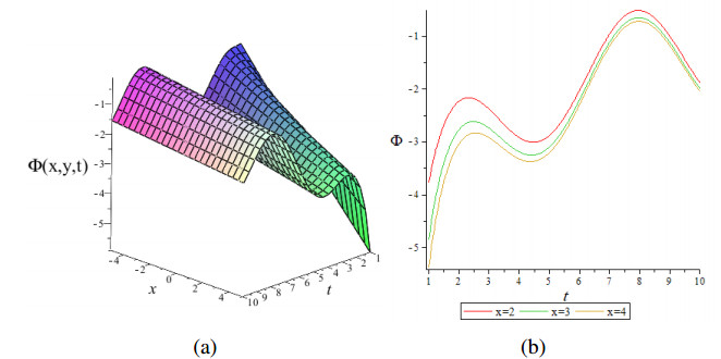
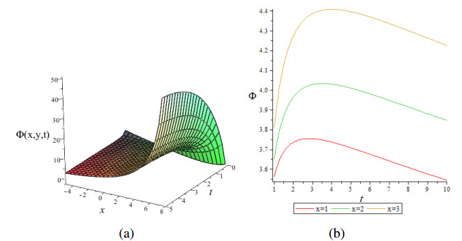
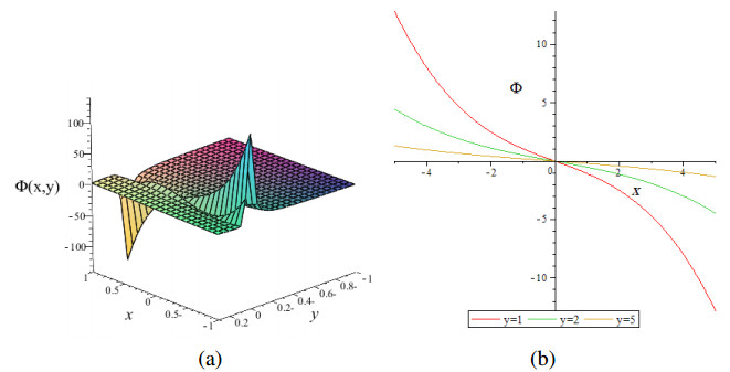
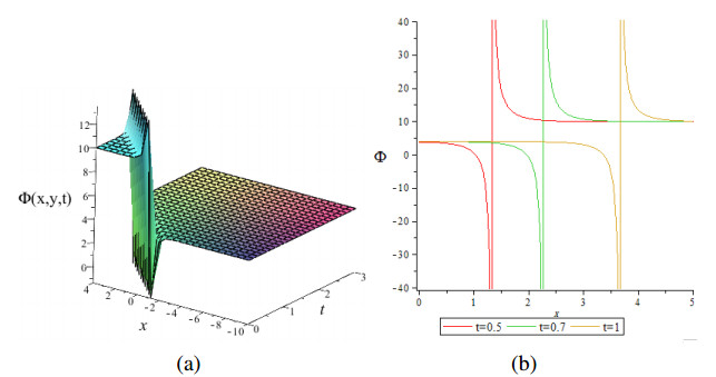
In this paper, we attempt to obtain exact and novel solutions for Date-Jimbo-Kashiwara-Miwa equation (DJKM) via two different techniques: Lie symmetry analysis and generalized Kudryashov method (GKM). This equation has applications in plasma physics, fluid mechanics, and other fields. The Lie symmetry method is applied to reduce the governing equation to five different ordinary differential equations (ODEs). GKM is used to obtain general and various periodic solutions. These solutions have different behaviors such as kink wave, anti-kink wave, double soliton, and single wave solution. The physical behavior of the solutions was reviewed through 2-D and 3-D graphs.

Keywords:

Citation: Ahmed A. Gaber, Abdul-Majid Wazwaz. Dynamic wave solutions for (2+1)-dimensional DJKM equation in plasma physics[J]. AIMS Mathematics, 2024, 9(3): 6060-6072. doi: 10.3934/math.2024296

Related Papers:

[1]	Yuanqing Xu, Xiaoxiao Zheng, Jie Xin . New non-traveling wave solutions for (3+1)-dimensional variable coefficients Date-Jimbo-Kashiwara-Miwa equation. AIMS Mathematics, 2021, 6(3): 2996-3008. doi: 10.3934/math.2021182
[2]	Ajay Kumar, Esin Ilhan, Armando Ciancio, Gulnur Yel, Haci Mehmet Baskonus . Extractions of some new travelling wave solutions to the conformable Date-Jimbo-Kashiwara-Miwa equation. AIMS Mathematics, 2021, 6(5): 4238-4264. doi: 10.3934/math.2021251
[3]	Chaudry Masood Khalique, Oke Davies Adeyemo, Kentse Maefo . Symmetry solutions and conservation laws of a new generalized 2D Bogoyavlensky-Konopelchenko equation of plasma physics. AIMS Mathematics, 2022, 7(6): 9767-9788. doi: 10.3934/math.2022544
[4]	Mobeen Munir, Muhammad Athar, Sakhi Sarwar, Wasfi Shatanawi . Lie symmetries of Generalized Equal Width wave equations. AIMS Mathematics, 2021, 6(11): 12148-12165. doi: 10.3934/math.2021705
[5]	Jamilu Sabi'u, Sekson Sirisubtawee, Surattana Sungnul, Mustafa Inc . Wave dynamics for the new generalized (3+1)-D Painlevé-type nonlinear evolution equation using efficient techniques. AIMS Mathematics, 2024, 9(11): 32366-32398. doi: 10.3934/math.20241552
[6]	Yanxia Hu, Qian Liu . On traveling wave solutions of a class of KdV-Burgers-Kuramoto type equations. AIMS Mathematics, 2019, 4(5): 1450-1465. doi: 10.3934/math.2019.5.1450
[7]	Tamara M. Garrido, Rafael de la Rosa, Elena Recio, Almudena P. Márquez . Conservation laws and symmetry analysis of a generalized Drinfeld-Sokolov system. AIMS Mathematics, 2023, 8(12): 28628-28645. doi: 10.3934/math.20231465
[8]	Yuqiang Feng, Jicheng Yu . Lie symmetry analysis of fractional ordinary differential equation with neutral delay. AIMS Mathematics, 2021, 6(4): 3592-3605. doi: 10.3934/math.2021214
[9]	Hammad Alotaibi . Solitary waves of the generalized Zakharov equations via integration algorithms. AIMS Mathematics, 2024, 9(5): 12650-12677. doi: 10.3934/math.2024619
[10]	Gaukhar Shaikhova, Bayan Kutum, Ratbay Myrzakulov . Periodic traveling wave, bright and dark soliton solutions of the (2+1)-dimensional complex modified Korteweg-de Vries system of equations by using three different methods. AIMS Mathematics, 2022, 7(10): 18948-18970. doi: 10.3934/math.20221043

Abstract

1. Introduction

1.1. Overview

Many physical phenomena, in the fields of sound and electrical waves, heat transfer, mechanics, and optics can be described through partial differential equations. Therefore, we can say that the study of mathematical physics depends primarily on the study of partial differential equations. During previous decades, many methods were developed to reduce and solve partial differential equations, including Symmetry method ^[1,2,3,4], scattering transformation ^[5], Tanh method ^[6], the homogeneous balance method ^[7], Aboodh transform decomposition method ^[8], ( $G^{\prime}/G$ , $1/G$ )-expansion method ^[9], Exp-function method ^[10], Generalized He's Exp-function method ^[11], Kudryashov method ^[12], and Generalized Kudryashov method ^[13]. Consider the nonlinear (2+1)-dimensional Date-Jimbo-Kashiwara-Miwa (DJKM) equation ^[14,15] in the following form:

$\begin{equation} \Phi_{xxxxy}+4\Phi_{xxy}\Phi_{x}+2\Phi_{xxx}\Phi_{y}+6\Phi_{xy}\Phi_{xx} +\Phi_{yyy}-2\Phi_{xxt} = 0, \end{equation}$

(1)

where $\Phi = \Phi(x, y, t).$ DJKM describes the wave diffusion of physical-quantity, and it has certain applications in plasma physics ^[16,17]. This equation was presented by Jimbo and Miwa as second formulas for Kadomtsev-Petviashvili hierarchy.

1.2. Related literatures

There is a wealth of literature related to this governing equation such as: Bibi and Ahmad ^[14] who employed the symmetry method to reduce the governing equation to another equation of lower order and obtained its exact solutions. The exp( $-\phi$ ( $\xi$ ))-Expansion Method was utilized by Sajid and Akram ^[14] for obtaining traveling wave solutions for Eq (1). Halder et al. ^[18] used the Lie symmetry analysis and singularity method to study one type of the governing equation. Wazwaz ^[19] studied the integrability of this equation and obtained multiple soliton solutions by using Painlevé analysis and Hirota's method. Akram et al. ^[16] applied the extended direct algebraic method to obtain exact solutions for the governing equation.

1.3. Main idea

The previous literature led us to determine the study of the governing equation to apply the Lie symmetry method and the Generalized Kudryashov method. Our main objective of this paper is to convert the governing equation to several distinct ordinary differential equations (ODE). We then solve the resulting ODEs to obtain exact and novel wave solutions for the governing equation. As a result, we can show the dynamic behavior of wave solutions in 2-D and 3-D plots.

2. Lie symmetry method

In this part, the Lie symmetry method ^[20,21,22] is used to deduce the similarity reductions for the governing equation, so the one-parameter Lie symmetry of infinitesimal variables is shown as follows:

$\begin{align*} t^{\ast} & = t+\varepsilon A(t,x,y,\Phi)+o(\varepsilon^{2}),\text{ }x^{\ast } = x+\varepsilon B(t,x,y,\Phi)+o(\varepsilon^{2}),\nonumber\\ y^{\ast} & = y+\varepsilon C(t,x,y,\Phi)+o(\varepsilon^{2}),\text{ } \Phi^{\ast} = \Phi+\varepsilon E(t,x,y,\Phi)+o(\varepsilon^{2}), \end{align*}$

(2)

where $\varepsilon$ is the one parameter Lie group, $A, \; B, \; C$ and $E$ are infinitesimal variables and $t, \; x$ and $y$ are independent variables of the function $\Phi.$

The vector generator $\chi$ is related to the above-mentioned group transformations which can be written as the following expression:

$\begin{equation} \chi = A\frac{\partial}{\partial t}+B\frac{\partial}{\partial x}+C\frac {\partial}{\partial y}+E\frac{\partial}{\partial\Phi}, \end{equation}$

(3)

when the following invariance condition is satisfied:

$\begin{equation} \Gamma^{(3)}(\Delta) = 0, \end{equation}$

(4)

where $\Delta$ represents Eq (1) and $\Gamma^{(3)}$ is the third order prolongation^[23,24] of the operator V

$\begin{align*} \Gamma^{(3)} & = \chi+E_{[x]}\frac{\partial}{\partial\Phi_{x}}+E_{[y]} \frac{\partial}{\partial\Phi_{y}}+E_{[xy]}\frac{\partial}{\partial\Phi_{xy} }+E_{[xxx]}\frac{\partial}{\partial\Phi_{xxx}}+E_{[xxy]}\frac{\partial }{\partial\Phi_{xxy}}\nonumber\\ & +E_{[xxt]}\frac{\partial\Phi}{\partial\Phi_{xxt}}+E_{[xxy]}\frac{\partial }{\partial\Phi_{xxy}}+E_{[xxxy]}\frac{\partial}{\partial\Phi_{xxxy}} +E_{[yyy]}\frac{\partial}{\partial\Phi_{yyy}}, \end{align*}$

(5)

where the components $E_{[x]}, E_{[xx]}, \; E_{[xyy]}, \; E_{[y]}, \; E_{[xy]}....$ can be determined from the following expressions:

$\begin{align*} E_{[x]} & = D_{x}E-\Phi_{t}D_{x}A-\Phi_{x}D_{x}B-\Phi_{y}D_{x}C,\nonumber\\ E_{[y]} & = D_{y}E-\Phi_{t}D_{y}A-\Phi_{x}D_{y}B-\Phi_{y}D_{y}C,\nonumber\\ \text{ }E_{[xx]} & = D_{x}E_{[x]}-\Phi_{xt}D_{x}A-\Phi_{xx}D_{x}B-\Phi _{xy}D_{x}C,\nonumber\\ \text{ }E_{[xy]} & = D_{y}E_{[x]}-\Phi_{xt}D_{y}A-\Phi_{xx}D_{y}B-\Phi _{xy}D_{y}C,\nonumber\\ \text{ }E_{[yy]} & = D_{y}E_{[y]}-\Phi_{xt}D_{y}A-\Phi_{xx}D_{y}B-\Phi _{xy}D_{y}C,\nonumber\\ E_{[xxxy]} & = D_{y}E_{[xxx]}-\Phi_{xxxt}D_{y}A-\Phi_{xxxx}D_{y}B-\Phi _{xxxy}D_{y}C. \end{align*}$

(6)

Substituting (1) into Eq (4), yields an identity components $A_{x}, A_{xx}, \; B_{t}, B_{x}, ....$ and adding the coefficients of $\Phi_{x, x, t}$ , $\Phi_{y, y, y}$ , ... and equating them to zero, then the infinitesimals $A, B, C$ and $E$ are obtained from the following equations:

$A_{x} = A_{y} = A_{\Phi} = 0,$

$B_{y} = B_{\Phi} = 0,B_{x} = \frac{1}{4}A_{t},$

$C_{x} = B_{\Phi} = 0,\text{ }C_{z} = \frac{1}{2}A_{t},$

$\begin{equation} E_{x} = \frac{-1}{2}C_{t},\text{ }E_{\Phi} = \frac{-1}{4}A_{t},\text{ }E_{y} = \frac{-1}{2}B_{t}. \end{equation}$

(7)

solving the system of Eq (7), we get

$\begin{align*} A & = g_{1}(t),\text{ }B = \frac{1}{4}g_{1}^{\prime}x+g_{3}(t),\text{ }C = \frac{1}{2}g_{1}^{\prime}y+g_{2}(t),\text{ }\nonumber\\ E & = \frac{-1}{4}g_{1}^{\prime}\Phi-\frac{1}{4}xyg_{1}^{\prime\prime} -yg_{2}^{\prime}-\frac{1}{2}xg_{3}^{\prime}+g_{4}(t). \end{align*}$

(8)

The vector field operator $V$ of Eq (8) can be presented as

$\begin{equation} V = V_{1}(c_{1})+V_{2}(c_{2})+V_{3}(c_{3})+V_{4}(c_{4}), \end{equation}$

(9)

where

$\begin{align*} V_{1} & = g_{1}(t)\left( \frac{\partial}{\partial t}+\frac{1}{4} x\frac{\partial}{\partial x}+\frac{1}{2}y\frac{\partial}{\partial y}-\frac {1}{4}\Phi\frac{\partial}{\partial\Phi}\right) -\frac{1}{4}xyg_{1} ^{\prime\prime}\frac{\partial}{\partial\Phi},\nonumber\\ V_{2} & = g_{2}(t)\frac{\partial}{\partial y}-y\alpha_{2}^{\prime} \frac{\partial}{\partial\Phi},\text{ }V_{3} = g_{3}(t)\frac{\partial }{\partial x}-\frac{1}{2}g_{3}^{\prime}\frac{\partial}{\partial\Phi},\text{ }V_{4} = g_{4}(t)\frac{\partial}{\partial\Phi}. \end{align*}$

(10)

The Lie-bracket $[V_{i}, V_{j}] = V_{i}V_{j}-V_{j}V_{i}$ is used for obtaining the commutator relations which are shown in Table 1, where

$\begin{align*} l_{1} & = g_{1}g_{2}^{\prime}-\frac{1}{2}g_{2}g_{1}^{\prime},\text{ } l_{2} = \frac{-1}{4}(g_{2}^{\prime}g_{1}^{\prime}+2g_{1}g_{2}^{\prime\prime }-g_{2}g_{1}^{\prime\prime})x,\nonumber\\ l_{3} & = g_{1}g_{3}^{\prime}-\frac{1}{4}g_{3}g_{1}^{\prime},\text{ } l_{4} = \frac{-1}{4}(g_{3}^{\prime}g_{1}^{\prime}+4g_{1}g_{3}^{\prime\prime }-g_{3}g_{1}^{\prime\prime})y,\nonumber\\ l_{5} & = \frac{1}{4}(4g_{1}g_{4}^{\prime}+g_{4}g_{1}^{\prime}),\text{ } l_{6} = \frac{-1}{2}(2g_{2}g_{3}^{\prime}-g_{3}g_{2}^{\prime}). \end{align*}$

(11)

Table 1. The commutator table.

	$V_{1}$	$V_{2}$	$V_{3}$	$V_{4}$
$V_{1}$	$0$	$l_{1}\frac{\partial}{\partial y}+l_{2}\frac{\partial }{\partial\Phi}$	$l_{3}\frac{\partial}{\partial x}+a_{4}\frac{\partial }{\partial\Phi}$	$l_{5}\frac{\partial}{\partial\Phi}$
$V_{2}$	-( $l_{1}\frac{\partial}{\partial y}+l_{2}\frac{\partial} {\partial\Phi})$	$0$	$l_{6}\frac{\partial}{\partial\Phi}$	$0$
$V_{3}$	-( $l_{3}\frac{\partial}{\partial x}+l_{4}\frac{\partial} {\partial\Phi})$	- $l_{6}\frac{\partial}{\partial\Phi}$	$0$	$0$
$V_{4}$	$-l_{5}\frac{\partial}{\partial\Phi}$	- $l_{6}\frac{\partial }{\partial\Phi}$	$0$	$0$

| Show Table

DownLoad: CSV

3. Reductions and closed form solutions

To obtain new independent variables, we utilize the characteristic equation as follows:

$\begin{equation} \frac{dt}{A(t,x,y,\Phi)} = \frac{dx}{B(t,x,y,\Phi)} = \frac{dy}{C(t,x,y,\Phi )} = \frac{d\Phi}{E(t,x,y,\Phi)}. \end{equation}$

(12)

Case I. Using $V_{1}$ where $g_{1}(t) = t^{2},$ Eq (12) takes the following form:

$\begin{equation} \frac{dt}{t^{2}} = \frac{dx}{\frac{1}{2}tx} = \frac{dy}{ty} = \frac{d\Phi}{\frac {-1}{2}t\Phi}. \end{equation}$

(13)

The similarity solution of Eq (1) takes the form

$\begin{equation} \Phi(t,x,y) = \frac{1}{\sqrt{t}}F(\zeta,\eta)-\frac{xy}{2t}, \end{equation}$

(14)

where $\zeta = \frac{x}{\sqrt{t}}, \; \eta = \frac{y}{t}.$ Substituting $\Phi$ in Eq (1) we get

$\begin{equation} F_{\eta\eta\eta}+6F_{\zeta\zeta}F_{\zeta\eta}+2F_{\zeta\zeta\zeta }F_{\eta}+4F_{\zeta\zeta\eta}F_{\zeta}+F_{\zeta\zeta\zeta\zeta\eta } = 0. \end{equation}$

(15)

The ordinary differential equations of Eq (15) take the following experssion:

$\begin{equation} h^{3}F^{\prime\prime\prime}(\theta)+6k^{3}hF^{\prime\prime^{2}}(\theta )+6k^{3}hF^{\prime\prime\prime}(\theta)F^{\prime}(\theta)+k^{4}hF^{\prime \prime\prime\prime\prime}(\theta) = 0, \end{equation}$

(16)

where $\theta = k\zeta+h\eta.$

To obtain the exact solution for Eq (16), we utilize generalized Kudryashov method (GKM) ^[11], given as follows:

$\begin{equation} F(\theta) = A_{0}+\sum\limits_{i=1}^m\frac{A_{i}}{(1+\phi (\theta))^{i}}, \end{equation}$

(17)

where $\phi(\theta)$ is the solution for the following Ricati equation $\phi^{\prime}(\theta) = A+B\phi(\theta)+C\phi^{2}(\theta).$ For simplicity, we take $i = 1$ and substitute Eq (17) into Eq (16) then to obtain

$\begin{equation} h = \pm\sqrt{4AC-B^{2}}k^{2},\text{ }A_{1} = 2k(C-B+A),\text{ }k\text{ and }A_{0}\text{ are arbitrary constant.} \end{equation}$

(18)

Substituting Eq (18) into Eqs (14) and (17), the exact solutions of Eq (1) can be expressed as

Set 1. $A\neq0, B\neq0, C\neq0.$

$\begin{equation} \Phi(t,x,y) = \frac{1}{\sqrt{t}}\left( A_{0}+\frac{2k(C-B+A)}{{\Large [} \frac{-B}{2C}\text{+}\frac{\sqrt{4AC-B^{2}}}{2C}\tan\text{(}\frac{1} {2}\text{(}\sqrt{4AC-B^{2}}\theta\text{))}+1{\LARGE ]}}\right) -\frac{xy} {2t}, \end{equation}$

(19)

where $\theta = k\frac{x}{\sqrt{t}}+\sqrt{4AC-B^{2}}k^{2}\frac{y}{t}.$

Set 2. $A = \frac{-1}{2}, B = 0, C = \frac{-1}{2}.$

$\begin{equation} \Phi(t,x,y) = \frac{1}{\sqrt{t}}\left( A_{0}+\frac{-2k}{\cot(\theta)\pm \csc(\theta)+1}\right) -\frac{xy}{2t}, \end{equation}$

(20)

where $\theta = k\frac{x}{\sqrt{t}}+2k^{2}\frac{y}{t}.$

Case II. Substituting $V_{1}$ in Eq (12) where $g_{1}(t) = t,$ then Eq (12) is expressed as follows:

$\begin{equation} \frac{dt}{t} = \frac{dx}{\frac{1}{4}x} = \frac{dy}{\frac{1}{2}y} = \frac{d\Phi }{\frac{-1}{4}\Phi}. \end{equation}$

(21)

Then the invariants are presented by $\zeta = \frac{x}{t^{\frac{1}{4}}}, \; \eta = \frac{y}{t^{\frac{1}{2}}}$ and $\Phi(t, x, y) = \frac{1}{t^{\frac{1}{4}} }F(\zeta, \eta).$ Further Eq (1) is reduced to the following form:

$\begin{align*} \frac{3}{2}F_{\zeta\zeta}+\frac{1}{2}\zeta F_{\zeta\zeta\zeta}+\eta F_{\eta\eta\eta}+F_{\eta\eta\eta}+6F_{\zeta\zeta}F_{\zeta\eta}+ 4F_{\zeta}F_{\zeta\zeta\eta}+2F_{\zeta\zeta\zeta}F_{\eta}+F_{\zeta \zeta\zeta\zeta\eta} = 0. \end{align*}$

(22)

For reducing Eq (22) to ODE we have two subcases:

Subcase (a). Using the scaling transformation in Eq (22)

$\begin{equation} F = e^{\epsilon}\text{ }\overset{-}{F},\text{ }\zeta = e^{\epsilon_{1}}\text{ }\overset{-}{\zeta},\text{ }\eta = e^{\epsilon_{2}}\text{ }\eta. \end{equation}$

(23)

Substituting from Eq (23) into Eq (22) we have $2\epsilon_{1} = \epsilon _{2} = -2\epsilon.$

The characteristic is given as

$\begin{equation} \frac{2d\zeta}{\zeta} = \frac{d\eta}{\eta} = \frac{-2dF}{F}. \end{equation}$

(24)

The invariant variables can be written as

$\begin{equation} \theta = \frac{\zeta^{2}}{\eta},\text{ }f = \frac{1}{\zeta^{2}}F(\theta). \end{equation}$

(25)

The ODE of Eq (22) is provided by

$\begin{align*} -\theta^{2}f^{\prime\prime\prime}-6f^{\prime\prime}-6\theta f^{\prime }-48\theta f^{\prime\prime^{2}}-48\theta ff^{\prime}-48f^{\prime} f^{\prime\prime\prime}-16f^{\prime}f^{\prime\prime\prime}-80\theta f^{\prime\prime\prime} -60f^{\prime\prime\prime}-16\theta^{2}f^{\prime\prime\prime\prime\prime} = 0. \end{align*}$

(26)

To obtain the exact solutions of Eq (26), we suppose that the solution of Eq (26) has the form

$\begin{equation} f(\theta) = A_{0}+\sum\limits_{j=1}^nA_{j}\theta^{j}. \end{equation}$

(27)

For simplicity, we take $j = 2$ , substitute Eq (27) into Eq (26), then the closed form solution of Eq (1) takes the expression

$\begin{equation} \Phi(x,y) = A_{0}+A_{1}\frac{x}{y}-\frac{1}{16}\frac{x^{3}}{y^{2}}, \end{equation}$

(28)

where $A_{0}$ and $A_{1}$ are arbitrary constant.

Subcase (b). Utilizing symmetry method for Eq (22), we obtained the infinitesimals of Eq (22) as follows:

$\begin{equation} \tau = \frac{1}{2}c_{1}\zeta+c_{2},\text{ }\beta = c_{1}\eta+c_{3},\text{ }\psi = \frac{-1}{2}(F+xy)c_{1}-\frac{1}{4}\eta c_{2}-\frac{1}{4}\zeta c_{3}. \end{equation}$

(29)

The vector field of Eq (22) can take the form

$\begin{equation} \chi = \chi_{1}(c_{1})+\chi_{2}(c_{2})+\chi_{3}(c_{3}), \end{equation}$

(30)

where

$\begin{equation} \chi_{1} = \frac{1}{2}\zeta\frac{\partial}{\partial\zeta}+\frac{\partial }{\partial\eta}-\frac{1}{2}(F+xy)\frac{\partial}{\partial F},\text{ }\chi _{2} = \frac{\partial}{\partial\zeta}-\frac{1}{4}\eta\frac{\partial}{\partial F},\text{ }\chi_{3} = \frac{\partial}{\partial\eta}-\frac{1}{4}\zeta \frac{\partial}{\partial F}. \end{equation}$

(31)

Using $\chi_{2}+w\chi_{3}$ , the characteristic equation is yielded

$\begin{equation} \frac{d\zeta}{1} = \frac{d\eta}{w} = \frac{dF}{-\frac{1}{4}\eta-\frac{w}{4}\zeta }. \end{equation}$

(32)

The similarity solution for Eq (22) takes the form

$\begin{equation} F(\zeta,\eta) = f(\theta)-\frac{1}{4}\eta\zeta,\text{ where }\theta = \eta-w\zeta. \end{equation}$

(33)

The reduced ODE can take the expression

$\begin{equation} f^{\prime\prime\prime}(\theta)-6w^{3}f^{\prime\prime2}(\theta)-6w^{3} f^{\prime}(\theta)f^{\prime\prime\prime}(\theta)+w^{4}f^{\prime\prime \prime\prime\prime}(\theta) = 0. \end{equation}$

(34)

Utilizing GKM in the previous case, the closed-form solution of Eq (34) is shown as

$\begin{equation} f(\theta) = A_{0}+\frac{A_{1}}{1+\phi(\theta)}+\frac{A_{2}}{(1+\phi(\theta ))^{2}}. \end{equation}$

(35)

Substituting Eq (35) into Eq (34), collecting the coefficients of derivative $\phi(\theta)$ and solving the algebraic equations, we obtain the values of $A_{0}$ and $A_{1}$

$\begin{equation} A_{1} = \frac{-2(A+C-B)}{(4AC-B^{2})^{\frac{1}{4}}},\text{ }w = \frac {1}{(4AC-B^{2})^{\frac{1}{4}}},\text{ }A_{0},\text{ }A_{2}\text{ are arbitrary.} \end{equation}$

(36)

Set 1. $A\neq0, B\neq0, C\neq0.$

$\begin{align*} \Phi(t,x,y) & = \frac{1}{t^{\frac{1}{4}}}\left( A_{0}+\frac{A_{1} }{{\Large [}\frac{-B}{2C}\text{+}\frac{\sqrt{4AC-B^{2}}}{2C}\tan\text{(} \frac{1}{2}\text{(}\sqrt{4AC-B^{2}}\theta\text{))}+1{\LARGE ]}}\right. \nonumber\\ & \left. +\frac{A_{2}}{{\Large [}\frac{-B}{2C}\text{+}\frac{\sqrt{4AC-B^{2} }}{2C}\tan\text{(}\frac{1}{2}\text{(}\sqrt{4AC-B^{2}}\theta\text{))} +1{\LARGE ]}^{2}}\right) -\frac{y}{4\sqrt{t}}\frac{x}{t^{\frac{1}{4}}}, \end{align*}$

(37)

where $A_{1} = \frac{-2(A+C-B)}{(4AC-B^{2})^{\frac{1}{4}}}, \; \theta = \frac {y}{\sqrt{t}}+\frac{1}{(4AC-B^{2})^{\frac{1}{4}}}\frac{x}{t^{\frac{1}{4}}}.$

Set 2. $A = \frac{1}{2}, B = 0, C = \frac{1}{2}.$

$\begin{equation} \Phi(t,x,y) = \frac{1}{t^{\frac{1}{4}}}\left( A_{0}+\frac{A_{1}}{\csc (\theta)-\cot(\theta)+1}+\frac{A_{2}}{(\csc(\theta)-\cot(\theta)+1)^{2} }\right) -\frac{y}{4\sqrt{t}}\frac{x}{t^{\frac{1}{4}}}, \end{equation}$

(38)

where $A_{1} = \frac{-1}{2}, \; \theta = \frac{y}{\sqrt{t}}+\frac{x}{t^{\frac{1} {4}}}.$

Cases III. Using $\mathbf{w}V_{2}, V_{3}, V_{4}$ where $g_{2}(t), \; g_{3}(t), \; g_{4}(t)$ are constants, we get

$\begin{equation} \frac{dt}{0} = \frac{dx}{w} = \frac{dy}{1} = \frac{d\Psi}{1}. \end{equation}$

(39)

Using Eq (39), we obtain the invariant solutions

$\begin{equation} \Phi(t,x,y) = F(\zeta,\eta)+y,\text{ where }\zeta = t,\text{ }\eta = x-wy. \end{equation}$

(40)

Substituting Eq (40) into Eq (1) we get

$\begin{equation} 2F_{\zeta\eta\eta}+w^{3}F_{\eta\eta\eta}+6wF_{\eta\eta}^{2}+6wF_{\eta \eta\eta}F_{\eta}-2F_{\eta\eta\eta}+wF_{\eta\eta\eta\eta\eta } = 0. \end{equation}$

(41)

Utilizing transformation $\theta = k\zeta+h\eta$ , Eq (41) is reduced to the next equation

$\begin{equation} h^{2}(2k+hw^{3}-2h)F^{\prime\prime\prime}(\theta)+6wh^{4}F^{\prime\prime^{2} }(\theta)+6wh^{4}F^{\prime\prime\prime}(\theta)F^{\prime}(\theta )+wh^{5}F^{\prime\prime\prime\prime\prime}(\theta) = 0. \end{equation}$

(42)

The exact solutions of Eq (42) can be deduced by applying GKM in the previous method. Substituting Eq (17) into Eq (42) at $i = 1$ and collecting the coefficient of derivative $\phi(\theta),$ then equating this equations to zero, this equations is solved and the values of $A_{0}, \; A_{1}, w, h$ and $k$ are obtained as

$\begin{align*} k = \frac{1}{2}(4h^{2}wAC+4-w^{3}-h^{2}wB^{2}),\text{ }A_{1} = 2(C+A-B)h,\; \; A_{0},h,w\text{ are arbitrary.} \end{align*}$

(43)

The closed-form solutions of Eq (1) can be expressed as

Set 1. $A\neq0, B\neq0, C = 0.$

$\begin{equation} \Phi(t,x,y) = A_{0}+\frac{2(A-B)h}{\frac{-A}{B}\text{+}\frac{1}{B}\exp \text{(}B\text{ }\theta\text{)}+1}+y, \end{equation}$

(44)

where $k = \frac{1}{2}(4-w^{3}-h^{2}wB^{2}), \; \theta = kt+h(x-wy).$

Set 2. $A = 0, B\neq0, C\neq0.$

$\begin{equation} \Phi(t,x,y) = A_{0}+\frac{2(C-B)h\text{ }(C\exp\text{(}B\text{ }\theta \text{)}-1)}{B\exp\text{(}B\text{ }\theta\text{)}+C\exp\text{(}B\text{ } \theta\text{)}-1}+y, \end{equation}$

(45)

where $k = \frac{1}{2}(4-w^{3}-h^{2}wB^{2}), \; \theta = kt+h(x-wy).$

Cases IV. Utilizing $wV_{2}, V_{3},$ where $\alpha _{2}(t), \alpha_{3}(t)$ are constant, we obtain

$\begin{equation} \frac{dt}{0} = \frac{dx}{1} = \frac{dy}{w} = \frac{d\Psi}{0}. \end{equation}$

(46)

Using Eq (46), we obtain the invariant solutions

$\begin{equation} \Phi(t,x,y) = F(\zeta,\eta),\text{ where }\zeta = t,\text{ }\eta = x-wy. \end{equation}$

(47)

Substituting Eq (47) into Eq (1) we get

$\begin{equation} 2F_{\zeta\eta\eta}+w^{3}F_{\eta\eta\eta}++6wF_{\eta\eta}^{2}+6wF_{\eta \eta\eta}F_{\eta}+wF_{\eta\eta\eta\eta\eta} = 0. \end{equation}$

(48)

Taking the transformation $\theta = k\zeta+h\eta$ , Eq (48) is reduced to the form

(49)

The coveted exact solution of Eq (49) is given. Hence, by using Eq (17) in Eq (49), the solution for Eq (1) is provided as

Set 1. $A\neq0, B\neq0, C\neq0.$

$\begin{equation} \Phi(t,x,y) = A_{0}+\frac{2(C+A-B)h}{{\Large [}\frac{-B}{2C}+\frac {\sqrt{4AC-B^{2}}}{2C}\tan(\frac{1}{2}(\sqrt{4AC-B^{2}}\theta))+1{\LARGE ]}}, \end{equation}$

(50)

where $k = \frac{1}{2}(4h^{2}wAC+4-w^{3}-h^{2}wB^{2}), \; \theta = kt+h(x-wy).$

Set 2. $A = \frac{1}{2}, B = 0, C = \frac{-1}{2}.$

$\begin{equation} \Phi(t,x,y) = A_{0}-\frac{1}{2}\frac{h}{\coth(\theta)\pm\csc h(\theta)+1}, \end{equation}$

(51)

where $k = \frac{1}{2}(-h^{2}w+4-w^{3}), \; \theta = kt+h(x-wy).$

4. Results & discussion

In this section, we explain the dynamic behavior of the obtained solutions in Eqs (19), (20), (28), (37), (38), (44), (45) and compare these results with previous literatures.

The physical behavior of the solutions is illustrated in three-dimensional and two-dimensional forms. The solutions include trigonometric functions, hyperbolic functions, and expansion functions. The Maple software was used to review the solutions as follows:

In , presents wave solution of Eq (19) in 3-D and 2-D shapes with perfect numerical values of $A_{0} = 5, \; k = 0.1, \; A = 3, \; C = 2, \; B = -1$ at y = 1.

Figure 1. Wave solution of Eq (19) in 3-D and 2-D shapes.

DownLoad: Full-Size Img PowerPoint

In , the solution of Eq (28) shows the behavior of a single wave and it is presented through 3-D and 2-D graphs. The constants are chosen as follows: $A_{0} = 1, A_{2} = 1, \; k = 0.1, \; A = 3, \; C = 2, \; B = 3$ when $y = 1$ .

Figure 2. Single wave of Eq (28) in 3-D and 2-D graphs.

DownLoad: Full-Size Img PowerPoint

shows doubly soliton of Eq (37) in 3-D and 2-D shapes with perfect choice for values of $A_{0} = 0, \; A_{1} = 1$ .

Figure 3. Doubly soliton of Eq (37) in 3-D and 2-D shapes.

DownLoad: Full-Size Img PowerPoint

depicts the view anti-kink wave solution of Eq (44) in 3-D and 2-D graphs with a suitable choice of values $A_{0} = 3, w = -1, h = -3, A = 2, C = 0, B = 1$ with $y = 1.$

Figure 4. Anti-kink wave solution of Eq (44) in 3-D and 2-D graphs.

DownLoad: Full-Size Img PowerPoint

In , the solution of Eq (45) represents a kink wave solution in 3-D and 2-D plots with perfect simulation of the values $A_{0} \; = 1, \; h = 2, w = 1, \; z = 1, A = 0, \; C = -3, B = 1$ at $y = 1.$

Figure 5. Kink wave solution of Eq (45) in 3-D and 2-D plots.

DownLoad: Full-Size Img PowerPoint

The authors in ^[13] used the symmetry method and obtained a subcase from our infinitesimals. Then, they reduced the governing equation to one reduction case, but we obtained five reduction cases.

The authors in ^[14] used two different traveling wave methods to obtain exact solutions. However, they reduced the governing equation through an algebraic transformation. When comparing these solutions with our obtained solutions, it turned out that our solutions are novel solutions and show different physical behavior from other solutions.

5. Conclusions

In this paper, we applied the Lie symmetry method to obtain infinitesimals and vector fields. This led to reduce the governing equation to a new form of partial differential equations (PDEs). Then, by utilizing the symmetry method again and similarity transformation: the new form of PDEs has been converted instead of reduced to five different ODEs. The general exact wave solutions are obtained by using GKM. These solutions are represented in 2-D and 3-D graphs to show the physical properties of the solutions.

Use of AI tools declaration

The authors declare that they have not used Artificial Intelligence (AI) tools in the creation of this article.

Acknowledgment

The author (A. A. Gaber) would like to thank the Deanship of Scientific Research of Majmaah University for supporting this work under Project Number (R-2024-947).

Conflict of interest

The authors declare no conflicts of interest.

References

[1]	A. Gaber, A. Wazwaz, Symmetries and dynamic wave solutions for (3+1)-dimensional potential Calogero-Bogoyavlenskii-Schiff equation, J. Ocean Eng. Sci., in press. http://dx.doi.org/10.1016/j.joes.2022.05.018
[2]	A. Gaber, Solitary and periodic wave solutions of (2+1)-dimensions of dispersive long wave equations on shallow waters, J. Ocean Eng. Sci., 6 (2021), 292–298. http://dx.doi.org/10.1016/j.joes.2021.02.002 doi: 10.1016/j.joes.2021.02.002
[3]	A. Gaber, F. Alsharari, S. Kumar, Some closed-form solutions, conservation laws, and various solitary waves to the (2+1)-D potential B-K equation via Lie symmetry approach, Int. J. Mod. Phys. B, 36 (2022), 2250117. http://dx.doi.org/10.1142/S021797922250117X doi: 10.1142/S021797922250117X
[4]	Z. Zhao, L. He, Lie symmetry, nonlocal symmetry analysis, and interaction of solutions of a (2+1)-dimensional Kdv-Mkdv equation, Theor. Math. Phys., 206 (2021), 142–162. http://dx.doi.org/10.1134/S0040577921020033 doi: 10.1134/S0040577921020033
[5]	M. Ablowitz, D. Kaup, A. Newell, Coherent pulse propagation, a dispersive, irreversible phenomenon, J. Math. Phys., 15 (1974), 1852–1858. http://dx.doi.org/10.1063/1.1666551
[6]	A. Wazwaz, The extended tanh method for new compact and noncompact solutions for the KP-BBM and the ZK-BBM equations, Chaos Soliton. Fract., 38 (2008), 1505–1516. http://dx.doi.org/10.1016/j.chaos.2007.01.135 doi: 10.1016/j.chaos.2007.01.135
[7]	Z. Dimitrova, K. Vitanov, Homogeneous balance method and auxiliary equation method as particular cases of simple equations method, AIP Conf. Proc., 2321 (2021), 030004. http://dx.doi.org/10.1063/5.0043070 doi: 10.1063/5.0043070
[8]	K. Khan, A. Ali, M. Irfan, Z. Khan, Solitary wave solutions in time-fractional Korteweg-de Vries equations with power law kernel, AIMS Mathematics, 8 (2023), 792–814. http://dx.doi.org/10.3934/math.2023039 doi: 10.3934/math.2023039
[9]	M. Mamun Miah, H. Shahadat Ali, M. Ali Akbar, A. Seadawy, New applications of the two variable (G $^{\prime}$ /G, 1/G)-expansion method for closed form traveling wave solutions of integro-differential equations, J. Ocean Eng. Sci., 4 (2019), 132–143. http://dx.doi.org/10.1016/j.joes.2019.03.001 doi: 10.1016/j.joes.2019.03.001
[10]	M. Shakeel, Attaullah, N. Ali Shah, J. Chung, Modified exp-function method to find exact solutions of microtubules nonlinear dynamics models, Symmetry, 15 (2023), 360. http://dx.doi.org/10.3390/sym15020360 doi: 10.3390/sym15020360
[11]	A. Gaber, A. Wazwaz, M. Mousa, Similarity reductions and new exact solutions for (3+1)-dimensional B-B equation, Mod. Phys. Lett. B, 38 (2024), 2350243. http://dx.doi.org/10.1142/S0217984923502433 doi: 10.1142/S0217984923502433
[12]	S. Kumar, K. Nisar, M. Niwas, On the dynamics of exact solutions to a (3+1)-dimensional YTSF equation emerging in shallow sea waves: Lie symmetry analysis and generalized Kudryashov method, Results Phys., 48 (2023), 106432. http://dx.doi.org/10.1016/j.rinp.2023.106432 doi: 10.1016/j.rinp.2023.106432
[13]	A. Gaber, A. Aljohani, A. Ebaid, J. Tenreiro Machado, The generalized Kudryashov method for nonlinear space-time fractional partial differential equations of Burgers type, Nonlinear Dyn., 95 (2019), 361–368. http://dx.doi.org/10.1007/s11071-018-4568-4 doi: 10.1007/s11071-018-4568-4
[14]	K. Bibi, K. Ahmad, New exact solutions of date Jimbo Kashiwara Miwa equation using Lie symmetry groups, Math. Probl. Eng., 2021 (2021), 5533983. http://dx.doi.org/10.1155/2021/5533983 doi: 10.1155/2021/5533983
[15]	N. Sajid, G. Akram, The application of the exp(- $\Phi$ ( $\xi$ ))-expansion method for finding the exact solutions of two integrable equations, Math. Probl. Eng., 2018 (2018), 5191736. http://dx.doi.org/10.1155/2018/5191736 doi: 10.1155/2018/5191736
[16]	G. Akram, N. Sajid, M. Abbas, Y. Hamed, K. Abualnaja, Optical solutions of the Date-Jimbo-Kashiwara-Miwa equation via the extended direct algebraic method, J. Math., 2021 (2021), 5591016. http://dx.doi.org/10.1155/2021/5591016 doi: 10.1155/2021/5591016
[17]	A. Rashed, S. Mabrouk, A. Wazwaz, Forward scattering for non-linear wave propagation in (3+1)-dimensional Jimbo-Miwa equation using singular manifold and group transformation methods, Wave. Random Complex, 32 (2022), 663–675. http://dx.doi.org/10.1080/17455030.2020.1795303 doi: 10.1080/17455030.2020.1795303
[18]	A. Halder, A. Paliathanasis, R. Seshadri, P. Leach, Lie symmetry analysis and similarity solutions for the Jimbo-Miwa equation and generalisations, Int. J. Nonlin. Sci. Num., 21 (2020), 767–779. http://dx.doi.org/10.1515/ijnsns-2019-0164 doi: 10.1515/ijnsns-2019-0164
[19]	A. Wazwaz, New (3+1)-dimensional Date-Jimbo-Kashiwara-Miwa equations with constant and time-dependent coefficients: Painlevé integrability, Phys. Lett. A, 384 (2020), 126787. http://dx.doi.org/10.1016/j.physleta.2020.126787 doi: 10.1016/j.physleta.2020.126787
[20]	S. Kumar, K. Nisar, M. Niwas, On the dynamics of exact solutions to a (3+1)-dimensional YTSF equation emerging in shallow sea waves: Lie symmetry analysis and generalized Kudryashov method, Results Phys., 48 (2023), 106432. http://dx.doi.org/10.1016/j.rinp.2023.106432 doi: 10.1016/j.rinp.2023.106432
[21]	M. El-Sayed, G. Moatimid, M. Moussa, R. El-Shiekh, F. El-Shiekh, A. El-Satar, A study of integrability and symmetry for the (p+1)th Boltzmann equation via Painlevé analysis and Lie-group method, Math. Method. Appl. Sci., 38 (2015), 3670–3677. http://dx.doi.org/10.1002/mma.3307 doi: 10.1002/mma.3307
[22]	S. Ray, Vinita, Lie symmetry analysis, symmetry reductions with exact solutions, and conservation laws of (2+1)-dimensional Bogoyavlenskii-Schieff equation of higher order in plasma physics, Math. Method. Appl. Sci., 43 (2020), 5850–5859. http://dx.doi.org/10.1002/mma.6328 doi: 10.1002/mma.6328
[23]	Z. Zhao, Bäcklund transformations, nonlocal symmetry and exact solutions of a generalized (2+1)-dimensional Korteweg-de Vries equation, Chinese J. Phys., 73 (2021), 695–705. http://dx.doi.org/10.1016/j.cjph.2021.07.026 doi: 10.1016/j.cjph.2021.07.026
[24]	S. Tian, M. Xu, T. Zhang, A symmetry-preserving difference scheme and analytical solutions of a generalized higher-order beam equation, Proc. R. Soc. A, 477 (2021), 20210455. http://dx.doi.org/10.1098/rspa.2021.0455 doi: 10.1098/rspa.2021.0455

This article has been cited by:

1.	Rajveer Singh, Sachin Kumar, Lie symmetry analysis, closed-form solutions and dynamics for the kinetics of phase separation in iron (Fe–Cr–X (X=Mo, Cu)) based on ternary alloys, 2024, 112, 0924-090X, 20255, 10.1007/s11071-024-10112-0
2.	Ahmed A. Gaber, Ahmet Bekir, Integrability, Similarity Reductions and New Classes of Exact Solutions for (3+1)-D Potential Yu–Toda–Sasa–Fukuyama Equation, 2024, 23, 1575-5460, 10.1007/s12346-024-01090-0
3.	Amer Darweesh, Marwan Alquran, New algorithm for deriving rational form solutions in the generalized Date-Jimbo-Kashiwara-Miwa model, 2024, 99, 0031-8949, 105271, 10.1088/1402-4896/ad7a29
4.	Yunjia Song, Yanzhi Ma, Ben Yang, Zenggui Wang, Exact solutions and bifurcations for the (3+1)-dimensional generalized KdV-ZK equation, 2024, 99, 0031-8949, 075205, 10.1088/1402-4896/ad4e14
5.	Muhammad Amin S Murad, Hajar F Ismael, Tukur Abdulkadir Sulaiman, Various exact solutions to the time-fractional nonlinear Schrödinger equation via the new modified Sardar sub-equation method, 2024, 99, 0031-8949, 085252, 10.1088/1402-4896/ad62a6
6.	Weaam Alhejaili, Abdul-Majid Wazwaz, Samir A El-Tantawy, Extended new Painlevé integrable KdV–CBS equation: multiple shocks, lump, breathers, and other physical wave solutions, 2025, 100, 0031-8949, 015292, 10.1088/1402-4896/ad9fac
7.	Muhammad Zubair Raza, Muhammad Abdaal Bin Iqbal, Aziz Khan, D. K. Almutairi, Thabet Abdeljawad, Soliton solutions of the (2 + 1)-dimensional Jaulent-Miodek evolution equation via effective analytical techniques, 2025, 15, 2045-2322, 10.1038/s41598-025-87785-z
8.	José M. Escorcia, Erwin Suazo, On explicit solutions for coupled reaction-diffusion and Burgers-type equations with variable coefficients through a Riccati system, 2025, 0, 1937-1632, 0, 10.3934/dcdss.2025030

Reader Comments

Your name:*

Email:*
© 2024 the Author(s), licensee AIMS Press. This is an open access article distributed under the terms of the Creative Commons Attribution License (http://creativecommons.org/licenses/by/4.0)

通讯作者: 陈斌, bchen63@163.com

1.
沈阳化工大学材料科学与工程学院沈阳 110142

AIMS Mathematics

1.8 3.4

Metrics

Article views(1367) PDF downloads(113) Cited by(8)

Preview PDF

Download XML

Export Citation

Article outline

Show full outline

Figures and Tables

Figures(5) / Tables(1)

AIMS Mathematics

Dynamic wave solutions for (2+1)-dimensional DJKM equation in plasma physics

Related Papers:

Abstract

1. Introduction

1.1. Overview

1.2. Related literatures

1.3. Main idea

2. Lie symmetry method

3. Reductions and closed form solutions

4. Results & discussion

5. Conclusions

Use of AI tools declaration

Acknowledgment

Conflict of interest

References

This article has been cited by:

Reader Comments

通讯作者: 陈斌, bchen63@163.com

Metrics

Figures and Tables

Other Articles By Authors

Catalog

AIMS Mathematics

Dynamic wave solutions for (2+1)-dimensional DJKM equation in plasma physics

Related Papers:

Abstract

1. Introduction

1.1. Overview

1.2. Related literatures

1.3. Main idea

2. Lie symmetry method

3. Reductions and closed form solutions

4. Results & discussion

5. Conclusions

Use of AI tools declaration

Acknowledgment

Conflict of interest

References

This article has been cited by:

Reader Comments

通讯作者: 陈斌, bchen63@163.com

Metrics

Figures and Tables

Other Articles By Authors

Related pages

Tools

Export File

Citation

Format

Content

Catalog