Symmetry solutions and conservation laws of a new generalized 2D Bogoyavlensky-Konopelchenko equation of plasma physics

Chaudry Masood Khalique; Oke Davies Adeyemo; Kentse Maefo; Chaudry Masood Khalique; Oke Davies Adeyemo; Kentse Maefo

doi:10.3934/math.2022544

AIMS Mathematics

2022, Volume 7, Issue 6: 9767-9788. doi: 10.3934/math.2022544

Previous Article Next Article

Research article Special Issues

Symmetry solutions and conservation laws of a new generalized 2D Bogoyavlensky-Konopelchenko equation of plasma physics

International Institute for Symmetry Analysis and Mathematical Modelling, Department of Mathematical Sciences, North-West University, Mafikeng Campus, Private Bag X 2046, Mmabatho 2735, Republic of South Africa

Received: 03 December 2021 Revised: 05 February 2022 Accepted: 13 February 2022 Published: 17 March 2022
MSC : 35L65, 35B06

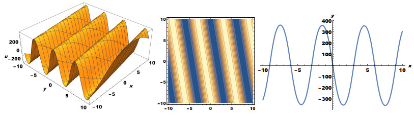
In physics as well as mathematics, nonlinear partial differential equations are known as veritable tools in describing many diverse physical systems, ranging from gravitation, mechanics, fluid dynamics to plasma physics. In consequence, we analytically examine a two-dimensional generalized Bogoyavlensky-Konopelchenko equation in plasma physics in this paper. Firstly, the technique of Lie symmetry analysis of differential equations is used to find its symmetries and perform symmetry reductions to obtain ordinary differential equations which are solved to secure possible analytic solutions of the underlying equation. Then we use Kudryashov's and $ (G'/G) $-expansion methods to acquire analytic solutions of the equation. As a result, solutions found in the process include exponential, elliptic, algebraic, hyperbolic and trigonometric functions which are highly important due to their various applications in mathematic and theoretical physics. Moreover, the obtained solutions are represented in diagrams. Conclusively, we construct conservation laws of the underlying equation through the use of multiplier approach. We state here that the results secured for the equation understudy are new and highly useful.
- two-dimensional generalized Bogoyavlensky-Konopelchenko equation,
- Lie point symmetries,
- analytic solutions,
- conservation laws
Citation: Chaudry Masood Khalique, Oke Davies Adeyemo, Kentse Maefo. Symmetry solutions and conservation laws of a new generalized 2D Bogoyavlensky-Konopelchenko equation of plasma physics[J]. AIMS Mathematics, 2022, 7(6): 9767-9788. doi: 10.3934/math.2022544

Related Papers:

Abstract

In physics as well as mathematics, nonlinear partial differential equations are known as veritable tools in describing many diverse physical systems, ranging from gravitation, mechanics, fluid dynamics to plasma physics. In consequence, we analytically examine a two-dimensional generalized Bogoyavlensky-Konopelchenko equation in plasma physics in this paper. Firstly, the technique of Lie symmetry analysis of differential equations is used to find its symmetries and perform symmetry reductions to obtain ordinary differential equations which are solved to secure possible analytic solutions of the underlying equation. Then we use Kudryashov's and $ (G'/G) $-expansion methods to acquire analytic solutions of the equation. As a result, solutions found in the process include exponential, elliptic, algebraic, hyperbolic and trigonometric functions which are highly important due to their various applications in mathematic and theoretical physics. Moreover, the obtained solutions are represented in diagrams. Conclusively, we construct conservation laws of the underlying equation through the use of multiplier approach. We state here that the results secured for the equation understudy are new and highly useful.

References

[1]	A. I. Morozov, Introduction to plasma dynamics, Boca Raton, Florida: CRC Press, 2012.
[2]	O. D. Adeyemo, T. Motsepa, C. M. Khalique, A study of the generalized nonlinear advection-diffusion equation arising in engineering sciences, Alex. Eng. J., 61 (2022), 185–194. https://doi.org/10.1016/j.aej.2021.04.066 doi: 10.1016/j.aej.2021.04.066
[3]	C. M. Khalique, O. D. Adeyemo, A study of (3+1)-dimensional generalized Korteweg-de Vries-Zakharov-Kuznetsov equation via Lie symmetry approach, Results Phys., 18 (2020), 103197. https://doi.org/10.1016/j.rinp.2020.103197 doi: 10.1016/j.rinp.2020.103197
[4]	A. Shafiq, C. M. Khalique, Lie group analysis of upper convected Maxwell fluid flow along stretching surface, Alex. Eng. J., 59 (2020), 2533–2541. https://doi.org/10.1016/j.aej.2020.04.017 doi: 10.1016/j.aej.2020.04.017
[5]	N. Benoudina, Y. Zhang, C. M. Khalique, Lie symmetry analysis, optimal system, new solitary wave solutions and conservation laws of the Pavlov equation, Commun. Nonlinear Sci. Numer. Simul., 94 (2021), 105560. https://doi.org/10.1016/j.cnsns.2020.105560 doi: 10.1016/j.cnsns.2020.105560
[6]	J. J. Li, G. Singh, O. A. İlhan, J. Manafian, Y. S. Gasimov, Modulational instability, multiple exp-function method, SIVP, solitary and cross-kink solutions for the generalized KP equation, AIMS Math., 6 (2021), 7555–7584. https://doi.org/10.3934/math.2021441 doi: 10.3934/math.2021441
[7]	E. Alimirzaluo, M. Nadjafikhah, J. Manafian, Some new exact solutions of (3+1)-dimensional Burgers system via Lie symmetry analysis, Adv. Differ. Equ., 2021 (2021), 1–17. https://doi.org/10.1186/s13662-021-03220-3 doi: 10.1186/s13662-021-03220-3
[8]	P. G. Estévez, J. D. Lejarreta, C. Sardón, Symmetry computation and reduction of a wave model in (2+1)-dimensions, Nonlinear Dyn., 87 (2017), 13–23. https://doi.org/10.1007/s11071-016-2997-5 doi: 10.1007/s11071-016-2997-5
[9]	B. Muatjetjeja, D. M. Mothibi, C. M. Khalique, Lie group classification a generalized coupled (2+1)-dimensional hyperbolic system, Discrete Contin. Dyn. Syst. Ser. S, 13 (2020), 2803–2812. https://doi.org/10.3934/dcdss.2020219 doi: 10.3934/dcdss.2020219
[10]	C. M. Khalique, I. Simbanefayi, Conserved quantities, optimal system and explicit solutions of a (1+1)-dimensional generalised coupled mKdV-type system, J. Adv. Res., 29 (2020), 159–166. https://doi.org/10.1016/j.jare.2020.10.002 doi: 10.1016/j.jare.2020.10.002
[11]	R. J. Leveque, Numerical methods for conservation laws, Basel: Birkhäuser, 1992. https://doi.org/10.1007/978-3-0348-8629-1
[12]	W. Sarlet, Comment on 'Conservation laws of higher order nonlinear PDEs and the variational conservation laws in the class with mixed derivatives', J. Phys. A Math. Theor., 43 (2010), 458001. https://doi.org/10.1088/1751-8113/43/45/458001 doi: 10.1088/1751-8113/43/45/458001
[13]	T. Motsepa, M. Abudiab, C. M. Khalique, A study of an extended generalized (2+1)-dimensional Jaulent-Miodek equation, Int. J. Nonlinear Sci. Numer. Simul., 19 (2018), 391–395. https://doi.org/10.1515/ijnsns-2017-0147 doi: 10.1515/ijnsns-2017-0147
[14]	N. H. Ibragimov, A new conservation theorem, J. Math. Anal. Appl., 333 (2007), 311–328. https://doi.org/10.1016/j.jmaa.2006.10.078 doi: 10.1016/j.jmaa.2006.10.078
[15]	C. M. Khalique, K. Maefo, A study on the (2+1)-dimensional first extended Calogero-Bogoyavlenskii-Schiff equation, Math. Biosci. Eng., 18 (2021), 5816–5835. https://doi.org/10.3934/mbe.2021293 doi: 10.3934/mbe.2021293
[16]	M. J. Ablowitz, P. A. Clarkson, Solitons, nonlinear evolution equations and inverse scattering, Cambridge University Press, 1991.
[17]	N. A. Kudryashov, Simplest equation method to look for exact solutions of nonlinear differential equations, Chaos Soliton. Fract., 24 (2005), 1217–1231. https://doi.org/10.1016/j.chaos.2004.09.109 doi: 10.1016/j.chaos.2004.09.109
[18]	C. H. Gu, Soliton theory and its application, Zhejiang Science and Technology Press, 1990.
[19]	Y. B. Zhou, M. L. Wang, Y. M. Wang, Periodic wave solutions to a coupled KdV equations with variable coefficients, Phys. Lett. A, 308 (2003), 31–36. https://doi.org/10.1016/S0375-9601(02)01775-9 doi: 10.1016/S0375-9601(02)01775-9
[20]	N. A. Kudryashov, N. B. Loguinova, Extended simplest equation method for nonlinear differential equations, Appl. Math. Comput., 205 (2008), 396–402. https://doi.org/10.1016/j.amc.2008.08.019 doi: 10.1016/j.amc.2008.08.019
[21]	R. Hirota, The direct method in soliton theory, Cambridge University Press, 2004.
[22]	P. J. Olver, Applications of Lie groups to differential equations, New York: Springer, 1993.
[23]	N. H. Ibragimov, CRC handbook of Lie group analysis of differential equations, Boca Raton, Florida: CRC Press, 1995.
[24]	N. H. Ibragimov, Elementary Lie group analysis and ordinary differential equations, New York: Wiley, 1999.
[25]	G. W. Wang, X. Q. Liu, Y. Y. Zhang, Symmetry reduction, exact solutions and conservation laws of a new fifth-order nonlinear integrable equation, Commun. Nonlinear Sci. Numer. Simul., 18 (2013), 2313–2320. https://doi.org/10.1016/j.cnsns.2012.12.003 doi: 10.1016/j.cnsns.2012.12.003
[26]	H. Z. Liu, J. B. Li, Lie symmetry analysis and exact solutions for the short pulse equation, Nonlinear Anal., 71 (2009), 2126–2133. https://doi.org/10.1016/j.na.2009.01.075 doi: 10.1016/j.na.2009.01.075
[27]	H. Z. Liu, J. B. Li, Q. X. Zhang, Lie symmetry analysis and exact explicit solutions for general Burgers' equation, J. Comput. Appl. Math., 228 (2009), 1–9. https://doi.org/10.1016/j.cam.2008.06.009 doi: 10.1016/j.cam.2008.06.009
[28]	S. N. Chow, J. K. Hale, Methods of bifurcation theory, New York: Springer, 1982. https://doi.org/10.1007/978-1-4613-8159-4
[29]	L. J. Zhang, C. M. Khalique, Classification and bifurcation of a class of second-order ODEs and its application to nonlinear PDEs, Discrete Contin. Dyn. Syst. Ser. S, 11 (2018), 759–772. https://doi.org/10.3934/dcdss.2018048 doi: 10.3934/dcdss.2018048
[30]	M. L. Wang, X. Z. Li, J. L. Zhang, The $ (G'/G)$-expansion method and travelling wave solutions for linear evolution equations in mathematical physics, Phys. Lett. A, 24 (2005), 1257–1268.
[31]	V. B. Matveev, M. A. Salle, Darboux transformations and solitons, Berlin: Springer, 1991.
[32]	Y. Chen, Z. Y. Yan, New exact solutions of (2+1)-dimensional Gardner equation via the new sine-Gordon equation expansion method, Chaos Soliton. Fract., 26 (2005), 399–406. https://doi.org/10.1016/j.chaos.2005.01.004 doi: 10.1016/j.chaos.2005.01.004
[33]	N. A. Kudryashov, One method for finding exact solutions of nonlinear differential equations, Commun. Nonlinear Sci. Numer. Simul., 17 (2012), 2248–2253. https://doi.org/10.1016/j.cnsns.2011.10.016 doi: 10.1016/j.cnsns.2011.10.016
[34]	O. I. Bogoyavlenskiĭ, Overturning solitons in new two-dimensional integrable equations, Math. USSR Izv., 34 (1990), 245–259.
[35]	B. G. Konopelchenko, Solitons in multidimensions: Inverse spectral transform method, Singapore: World Scientific, 1993.
[36]	M. V. Prabhakar, H. Bhate, Exact solutions of the Bogoyavlensky-Konoplechenco equation, Lett. Math. Phys., 64 (2003), 1–6. https://doi.org/10.1023/A:1024909327151 doi: 10.1023/A:1024909327151
[37]	S. S. Ray, On conservation laws by Lie symmetry analysis for (2+1)-dimensional Bogoyavlensky-Konopelchenko equation in wave propagation, Comput. Math. Appl., 74 (2017), 1158–1165. https://doi.org/10.1016/j.camwa.2017.06.007 doi: 10.1016/j.camwa.2017.06.007
[38]	F. Calogero, A method to generate solvable nonlinear evolution equations, Lett. Nuovo Cimento, 14 (1975), 443–447. https://doi.org/10.1007/BF02763113 doi: 10.1007/BF02763113
[39]	K. Toda, S. J. Yu, A study of the construction of equations in (2+1) dimensions, Inverse Probl., 17 (2001), 1053.
[40]	Q. Li, T. Chaolu, Y. H. Wang, Lump-type solutions and lump solutions for the (2+1)-dimensional generalized Bogoyavlensky-Konopelchenko equation, Comput. Math. Appl., 77 (2019), 2077–2085. https://doi.org/10.1016/j.camwa.2018.12.011 doi: 10.1016/j.camwa.2018.12.011
[41]	F. Y. Liu, Y. T. Gao, X. Yu, L. Q. Li, C. C. Ding, D. Wang, Lie group analysis and analytic solutions for a (2+1)-dimensional generalized Bogoyavlensky-Konopelchenko equation in fluid mechanics and plasma physics, Eur. Phys. J. Plus, 136 (2021), 1–14. https://doi.org/10.1140/epjp/s13360-021-01469-x doi: 10.1140/epjp/s13360-021-01469-x
[42]	J. Y. Yang, W. X. Ma, C. M. Khalique, Determining lump solutions for a combined soliton equation in (2+1)-dimensions, Eur. Phys. J. Plus, 135 (2020), 1–13. https://doi.org/10.1140/epjp/s13360-020-00463-z doi: 10.1140/epjp/s13360-020-00463-z
[43]	Y. Kosmann-Schwarzbach, B. Grammaticos, K. M. Tamizhmani, Integrability of nonlinear systems, Berlin, Heidelberg: Springer, 2004. https://doi.org/10.1007/b94605
[44]	S. T. Chen, W. X. Ma, Lump solutions of a generalized Calogero-Bogoyavlenskii-Schiff equation, Comput. Math. Appl., 76 (2018), 1680–1685. https://doi.org/10.1016/j.camwa.2018.07.019 doi: 10.1016/j.camwa.2018.07.019
[45]	N. A. Kudryashov, Analytical theory of nonlinear differential equations, Moskow-Igevsk, Institute of Computer Investigations, 2004.
[46]	I. S. Gradshteyn, I. M. Ryzhik, Table of integrals, series, and products, New York: Academic Press, 2007.
[47]	N. I. Akhiezer, Elements of the theory of elliptic functions, Providence, Rhode Island: American Mathematical Society, 1990.
[48]	N. A. Kudryashov, First integrals and general solution of the Fokas-Lenells equation, Optik, 195 (2019), 163135. https://doi.org/10.1016/j.ijleo.2019.163135 doi: 10.1016/j.ijleo.2019.163135
[49]	S. C. Anco, G. Bluman, Direct construction method for conservation laws of partial differential equations Part I: Examples of conservation law classifications, Eur. J. Appl. Math., 13 (2002), 545–566. https://doi.org/10.1017/S095679250100465X doi: 10.1017/S095679250100465X
[50]	S. C. Anco, G. Bluman, Direct construction method for conservation laws of partial differential equations Part II: General treatment, Eur. J. Appl. Math., 13 (2002), 567–585. https://doi.org/10.1017/S0956792501004661 doi: 10.1017/S0956792501004661
[51]	E. Noether, Invariante variationsprobleme, Nachr. Ges. Wiss. Göttingen Math. Phys. Kl., 1918 (1918), 235–257.

Reader Comments

Your name:*

Email:*
© 2022 the Author(s), licensee AIMS Press. This is an open access article distributed under the terms of the Creative Commons Attribution License (http://creativecommons.org/licenses/by/4.0)