Fixed-time synchronization problem of coupled delayed discontinuous neural networks via indefinite derivative method

Huijun Xiong; Chao Yang; Wenhao Li; Huijun Xiong; Chao Yang; Wenhao Li

doi:10.3934/era.2023084

Electronic Research Archive

2023, Volume 31, Issue 3: 1625-1640. doi: 10.3934/era.2023084

Previous Article Next Article

Research article Special Issues

Fixed-time synchronization problem of coupled delayed discontinuous neural networks via indefinite derivative method

School of Mathematics, Changsha University, Changsha 410022, China

Academic Editor: Dongshu Wang

Received: 18 September 2022 Revised: 13 January 2023 Accepted: 21 January 2023 Published: 31 January 2023

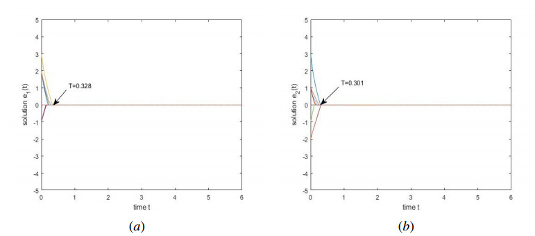
In this brief, we introduce a class of coupled delayed nonautonomous neural networks (CDNNs) with discontinuous activation function. Different from the conventional Lyapunov method, this brief uses the implementation of an indefinite derivative to deal with the nonautonomous system for the case that the topology between neurons is nonlinear coupling, and the system can achieve synchronization in fixed time by selecting the suitable control scheme. The settling time estimation of the system which can get rid of the dependence on the initial value is given. Finally, two examples are given to verify the correctness of the results in this paper.
- fixed-time synchronization (FTS),
- discontinuous neural networks,
- nonlinear coupling,
- indefinite derivative
Citation: Huijun Xiong, Chao Yang, Wenhao Li. Fixed-time synchronization problem of coupled delayed discontinuous neural networks via indefinite derivative method[J]. Electronic Research Archive, 2023, 31(3): 1625-1640. doi: 10.3934/era.2023084

Related Papers:

Abstract

In this brief, we introduce a class of coupled delayed nonautonomous neural networks (CDNNs) with discontinuous activation function. Different from the conventional Lyapunov method, this brief uses the implementation of an indefinite derivative to deal with the nonautonomous system for the case that the topology between neurons is nonlinear coupling, and the system can achieve synchronization in fixed time by selecting the suitable control scheme. The settling time estimation of the system which can get rid of the dependence on the initial value is given. Finally, two examples are given to verify the correctness of the results in this paper.

References

[1]	X. Liang, T. Yamaguchi, On the analysis of global and absolute stability of nonlinear continuous neural networks, Ieice Trans. Fund. Electr., 80 (1997), 223–229.
[2]	A. Guez, E. Protopopsecu, J. Barhen, On the stability, storage capacity, and design of nonlinear continuous neural networks, IEEE Trans. Syst. Man Cybernetics, 18 (1988), 80–87. https://doi.org/10.1109/21.87056 doi: 10.1109/21.87056
[3]	J. Hu, Synchronization conditions for chaotic nonlinear continuous neural networks, Chaos Solitons Fractals, 41 (2009), 2495–2501. https://doi.org/10.1016/j.chaos.2008.09.026 doi: 10.1016/j.chaos.2008.09.026
[4]	Z. Cai, L. Huang, Z. Wang, fixed-time stability criteria for discontinuous nonautonomous systems: Lyapunov method with indefinite derivative, IEEE Trans. Cybernetics, 41 (2009), 2495–2501.
[5]	H. Rostro-Gonzalez, B. Cessac, T. Vieville, Parameter estimation in spiking neural networks: A reverse-engineering approach, J. Neural Eng., 9 (2012), 26024–26037. https://doi.org/10.1088/1741-2560/9/2/026024 doi: 10.1088/1741-2560/9/2/026024
[6]	S. Smith, R. Escobedo, A deployed engineering design retrieval system using neural networks, Trans. Neural Networks, 8 (1997), 847–851. https://doi.org/10.1109/72.595882 doi: 10.1109/72.595882
[7]	C. Aouiti, F. Miaadi, Finite-time stabilization of neutral hopfield neural networks with mixed delays, Neural Process. Lett., 48 (2018), 1645–1669. https://doi.org/10.1007/s11063-018-9791-y doi: 10.1007/s11063-018-9791-y
[8]	Q. Li, J. Yu, B. Mu, X. Sun, BP neural network prediction of the mechanical properties of porous NiTi shape memory alloy prepared by thermal explosion reaction, Mater. Sci. Eng. A, 419 (2006), 214–217. https://doi.org/10.1016/j.msea.2005.12.027 doi: 10.1016/j.msea.2005.12.027
[9]	S. H. Strogatz, I. N. Stewart, Coupled oscillators and biological synchronization, Sci. Am., 269 (1993), 102–109. https://doi.org/10.1038/scientificamerican1293-102 doi: 10.1038/scientificamerican1293-102
[10]	Z. Cai, L. Huang, Z. Wang, X. Pan, S. Liu, Periodicity and multi-periodicity generated by impulses control in delayed Cohen–Grossberg-type neural networks with discontinuous activations, Neural Networks, 143 (2021), 230–245. https://doi.org/10.1016/j.neunet.2021.06.013 doi: 10.1016/j.neunet.2021.06.013
[11]	X. Yang, J. Cao, Finite-time stochastic synchronization of complex networks, Appl. Math. Model., 34 (2010), 3631–3641. https://doi.org/10.1016/j.apm.2010.03.012 doi: 10.1016/j.apm.2010.03.012
[12]	J. Cortes, Finite-time convergent gradient flows with applications to network consensus, Automatica, 42 (2006), 1993–2000. https://doi.org/10.1016/j.automatica.2006.06.015 doi: 10.1016/j.automatica.2006.06.015
[13]	M. R. Mufti, H. Afzal, F. Rehman, N. Ahmed, Stabilization and synchronization of 5-D memristor oscillator using sliding mode control, J. Chin. Inst. Eng., 41 (2018), 667–677. https://doi.org/10.1080/02533839.2018.1534558 doi: 10.1080/02533839.2018.1534558
[14]	S. Yang, C. Li, T. Huang, Finite-time stabilization of uncertain neural networks with distributed time-varying delays, Neural Comput. Appl., 28 (2017), 667–677. https://doi.org/10.1007/s00521-016-2421-6 doi: 10.1007/s00521-016-2421-6
[15]	L. Liu, J. Sun, Finite-time stabilization of linear systems via impulsive control, Int. J. Control, 81 (2008), 905–909. https://doi.org/10.1080/00207170701519060 doi: 10.1080/00207170701519060
[16]	L. Wang, F. Xiao, Finite-time consensus problems for networks of dynamic agents, IEEE Trans. Autom. Control, 55 (2007), 950–955. https://doi.org/10.1109/TAC.2010.2041610 doi: 10.1109/TAC.2010.2041610
[17]	M. Forti, P. Nistri, Global convergence of neural networks with discontinuous neuron activations, IEEE Trans. Circuits Syst., 50 (2003), 1421–1435. https://doi.org/10.1109/TCSI.2003.818614 doi: 10.1109/TCSI.2003.818614
[18]	M. Forti, P. Nistri, D. Papini, Global exponential stability and global convergence in finite time of delayed neural networks with infinite gain, IEEE Trans. Neural Networks, 16 (2005), 1449–1463. https://doi.org/10.1109/TNN.2005.852862 doi: 10.1109/TNN.2005.852862
[19]	M. Forti, M. Grazzini, P. Nistri, L. Pancioni, Generalized Lyapunov approach for convergence of neural networks with discontinuous or non-Lipschitz activations, Phys. D Nonlinear Phenom., 214 (2006), 88–99. https://doi.org/10.1016/j.physd.2005.12.006 doi: 10.1016/j.physd.2005.12.006
[20]	H. Wu, Y. Li, Existence and stability of periodic solution for BAM neural networks with discontinuous neuron activations, Comput. Math. Appl., 56 (2008), 1981–1993. https://doi.org/10.1016/j.camwa.2008.04.027 doi: 10.1016/j.camwa.2008.04.027
[21]	B. Wang, J. Jian, Stability and Hopf bifurcation analysis on a four-neuron BAM neural network with distributed delays, Commun. Nonlinear Sci. Numer. Simul., 15 (2010), 189–204. https://doi.org/10.1016/j.cnsns.2009.03.033 doi: 10.1016/j.cnsns.2009.03.033
[22]	L. Zhang, L. Huang, Z. Cai, Finite-time stabilization control for discontinuous time-delayed networks: New switching design, Neural Networks, 75 (2016), 84–96. https://doi.org/10.1016/j.neunet.2015.11.009 doi: 10.1016/j.neunet.2015.11.009
[23]	Z. Yi, G. Xu, X. Qin, Z. Jia, Improvement and application of transient chaos neural networks, Procedia Eng., 24 (2011), 479–483. https://doi.org/10.1016/j.proeng.2011.11.2680 doi: 10.1016/j.proeng.2011.11.2680
[24]	K. Wang, N. Michel, Robustness and perturbation analysis of a class of nonlinear systems with applications to neural networks, IEEE Trans. Circuits Syst., 41 (1994), 24–32. https://doi.org/10.1109/81.260216 doi: 10.1109/81.260216
[25]	L. Duan, L. Huang, Z. Cai, Existence and stability of periodic solution for mixed time-varying delayed neural networks with discontinuous activations, Neurocomputing, 123 (2014), 255–265. https://doi.org/10.1016/j.neucom.2013.06.038 doi: 10.1016/j.neucom.2013.06.038
[26]	C. Marcus, R. Westervelt, Stability of analog neural networks with delay, Phys. Rev. A, 39 (1989), 347–359. https://doi.org/10.1103/PhysRevA.39.347 doi: 10.1103/PhysRevA.39.347
[27]	H. Su, X. Wang, Z. Lin, Flocking of multi-agents with a virtual leader, IEEE Trans. Autom. Control, 54 (2009), 293–307. https://doi.org/10.1109/TAC.2008.2010897 doi: 10.1109/TAC.2008.2010897
[28]	G. Wen, Z. Duan, W. Ren, G. Chen, Distributed consensus of multi-agent systems with general linear node dynamics and intermittent communications, Int. J. Robust Nonlinear Control, 24 (2014), 2438–2457. https://doi.org/10.1002/rnc.3001 doi: 10.1002/rnc.3001
[29]	X. Shi, X. Sun, Y. Lv, Q. Lu, H. Wang, Cluster synchronization and rhythm dynamics in a complex neuronal network with chemical synapses, Int. J. Non-linear Mech., 70 (2015), 112–118. https://doi.org/10.1016/j.ijnonlinmec.2014.11.030 doi: 10.1016/j.ijnonlinmec.2014.11.030
[30]	X. Sun, J. Lei, M. Perc, J. Kurths, G. Chen, Burst synchronization transitions in a neuronal network of subnetworks, Chaos, 21 (2011), 016110. https://doi.org/10.1063/1.3559136 doi: 10.1063/1.3559136
[31]	W. Lu, T. Chen, New approach to synchronization analysis of linearly coupled ordinary differential systems, Phys. D Nonlinear Phenom., 213 (2006), 214–230. https://doi.org/10.1016/j.physd.2005.11.009 doi: 10.1016/j.physd.2005.11.009
[32]	H. Zhang, F. L. Lewis, A. Das, Optimal design for synchronization of cooperative systems: State feedback, observer and output feedback, IEEE Trans. Autom. Control, 56 (2011), 1948–1952. https://doi.org/10.1109/TAC.2011.2139510 doi: 10.1109/TAC.2011.2139510
[33]	Z. Wang, L. Huang, Y. Wang, Y. Zuo, Synchronization analysis of networks with both delayed and non-delayed couplings via adaptive pinning control method, Commun. Nonlinear Sci. Numer. Simul., 15 (2010), 4202–4208. https://doi.org/10.1016/j.cnsns.2010.02.001 doi: 10.1016/j.cnsns.2010.02.001
[34]	X. Li, X. Wang, G. Chen, Pinning a complex dynamical network to its equilibrium, IEEE Trans. Circuits Syst. I, 51 (2004), 2074–2087. https://doi.org/10.1109/TCSI.2004.835655 doi: 10.1109/TCSI.2004.835655
[35]	T. Chen, X. Liu, W. Lu, Pinning Complex Networks by a Single Controller, IEEE Trans. Circuits Syst. I, 54 (2006), 1317–1326. https://doi.org/10.1109/TCSI.2007.895383 doi: 10.1109/TCSI.2007.895383
[36]	A. E. Polyakov, D. V. Efimov, W. Perruquetti, Finite-time and fixed-time stabilization: Implicit Lyapunov function approach, Automatica, 51 (2015), 332–340. https://doi.org/10.1016/j.automatica.2014.10.082 doi: 10.1016/j.automatica.2014.10.082
[37]	J. P. Aubin, A. Cellina, Differential Inclusions: Set-Valued Maps and Viability Theory, Springer-Verlag, Berlin, Heidelberg, 1984. https://doi.org/10.1007/978-3-642-69512-4
[38]	J. P. Lasalle, The Stability of Dynamical Systems, Society for Industrial and Applied Mathematics, 1976.
[39]	A. F. Filippov, Differential Equations with Discontinuous Righthand Sides, Springer Dordrecht, 1988. https://doi.org/10.1007/978-94-015-7793-9
[40]	F. H. Clarke, Optimization and Nonsmooth Analysis, Society for Industrial and Applied Mathematics, 1990.
[41]	G. H. Hardy, Inequalities, 2nd edition, Cambridge University Press, 1988.
[42]	A. S. Abdulhussien, A. T. AbdulSaddaa, K. Iqbal, Automatic seizure detection with different time delays using SDFT and time-domain feature extraction, J. Biomed. Res., 36 (2022), 48-57. https://doi.org/10.7555/JBR.36.20210124 doi: 10.7555/JBR.36.20210124
[43]	Y. Zhang, C. Mu, Y. Zhang, Y. Feng, Heuristic dynamic programming-based learning control for discrete-time disturbed multi-agent systems, Control Theory Technol., 19 (2021), 339–353. https://doi.org/10.1007/s11768-021-00049-9 doi: 10.1007/s11768-021-00049-9
[44]	F. Miaadi, X. Li, Impulse-dependent settling-time for finite time stabilization of uncertain impulsive static neural networks with leakage delay and distributed delays, Math. Comput. Simul., 182 (2021), 259–276. https://doi.org/10.1016/j.matcom.2020.11.003 doi: 10.1016/j.matcom.2020.11.003
[45]	N. Garcia, C. Kawan, S. Yuksel, Ergodicity conditions for controlled stochastic nonlinear systems under information constraints: A volume growth approach, SIAM J. Control. Optim., 59 (2021), 534–560. https://doi.org/10.1137/20M1315920 doi: 10.1137/20M1315920

Reader Comments

Your name:*

Email:*
© 2023 the Author(s), licensee AIMS Press. This is an open access article distributed under the terms of the Creative Commons Attribution License (http://creativecommons.org/licenses/by/4.0)