Well-posedness of generalized Stokes-Brinkman equations modeling moving solid phases

Nisachon Kumankat; Kanognudge Wuttanachamsri; Nisachon Kumankat; Kanognudge Wuttanachamsri

doi:10.3934/era.2023085

Electronic Research Archive

2023, Volume 31, Issue 3: 1641-1661. doi: 10.3934/era.2023085

Previous Article Next Article

Research article

Well-posedness of generalized Stokes-Brinkman equations modeling moving solid phases

Department of Mathematics, School of Science, King Mongkut's Institute of Technology Ladkrabang, Bangkok 10520, Thailand

Received: 04 November 2022 Revised: 04 January 2023 Accepted: 12 January 2023 Published: 31 January 2023

Fluid flow through a free-fluid region and the adjacent porous medium has been studied in various problems, such as water flow in rice fields. For the problem with self-propelled solid phases, we provide a generalized Stokes equation for the free-fluid domain and the Brinkman equation in a macroscopic scale due to the movement of self-propelled solid phases rather than a single solid in the porous medium. The model is derived with the assumption that the porosity is not a constant. The porosity in the mathematical model varies depending on the propagation of the solid phases. These two models can be matched at the free-fluid/porous-medium interface and are developed for real world problems. We show the proof of the well-posedness of the discretized form of the weak formulation obtained from applying a mixed finite element scheme to the generalized Stokes-Brinkman equations. The proofs of the continuity and coercive property of the linear and bilinear functionals in the discretized equation are illustrated. We present the existence and uniqueness of the generalized Stokes-Brinkman equations for the numerical problem in two dimensions. The system of equations can be applied to fluid flow propelled by moving solid phases, such as mucus flow in the trachea.
- generalized Stokes-Brinkman equations,
- finite element approach,
- well-posedness,
- varied porosity,
- permeability tensor
Citation: Nisachon Kumankat, Kanognudge Wuttanachamsri. Well-posedness of generalized Stokes-Brinkman equations modeling moving solid phases[J]. Electronic Research Archive, 2023, 31(3): 1641-1661. doi: 10.3934/era.2023085

Related Papers:

Abstract

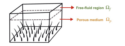
Fluid flow through a free-fluid region and the adjacent porous medium has been studied in various problems, such as water flow in rice fields. For the problem with self-propelled solid phases, we provide a generalized Stokes equation for the free-fluid domain and the Brinkman equation in a macroscopic scale due to the movement of self-propelled solid phases rather than a single solid in the porous medium. The model is derived with the assumption that the porosity is not a constant. The porosity in the mathematical model varies depending on the propagation of the solid phases. These two models can be matched at the free-fluid/porous-medium interface and are developed for real world problems. We show the proof of the well-posedness of the discretized form of the weak formulation obtained from applying a mixed finite element scheme to the generalized Stokes-Brinkman equations. The proofs of the continuity and coercive property of the linear and bilinear functionals in the discretized equation are illustrated. We present the existence and uniqueness of the generalized Stokes-Brinkman equations for the numerical problem in two dimensions. The system of equations can be applied to fluid flow propelled by moving solid phases, such as mucus flow in the trachea.

References

[1]	F. Basirat, P. Sharma, F. Fagerlund, A. Niemi, Experimental and modeling investigation of $\text{CO}_{2}$ flow and transport in a coupled domain of porous media and free flow, Int. J. Greenhouse Gas Control, 42 (2015), 461–470. https://doi.org/10.1016/j.ijggc.2015.08.024 doi: 10.1016/j.ijggc.2015.08.024
[2]	N. Oangwatcharaparkan, K. Wuttanachamsri, The flow in periciliary layer in human lungs with Navier-Stokes-Brinkman equations, Tamkang J. Math., 54 (2021). https://doi.org/10.5556/j.tkjm.54.2023.3738 doi: 10.5556/j.tkjm.54.2023.3738
[3]	K. Khanafer, K. Cook, A. Marafie, The role of porous media in modeling fluid flow within hollow fiber membranes of the total artificial lung, J. Porous Media, 15 (2012), 113–122. https://doi.org/10.1615/JPorMedia.v15.i2.20 doi: 10.1615/JPorMedia.v15.i2.20
[4]	H. B. Ly, H. L. Nguyen, M. N. Do, Finite element modeling of fluid flow in fractured porous media using unified approach, Vietnam J. Earth Sci., 43 (2020), 13–22. https://doi.org/10.15625/0866-7187/15572 doi: 10.15625/0866-7187/15572
[5]	K. Wuttanachamsri, L. Schreyer, Effects of cilia movement on fluid velocity: Ⅱ numerical solutions over a fixed domain, Transp. Porous Media, 134 (2020), 471–489. https://doi.org/10.1007/s11242-020-01455-4 doi: 10.1007/s11242-020-01455-4
[6]	S. Poopra, K. Wuttanachamsri, The velocity of PCL fluid in human lungs with Beaver and Joseph boundary condition by using asymptotic expansion method, Mathematics, 7 (2019), 567. https://doi.org/10.3390/math7060567 doi: 10.3390/math7060567
[7]	K. Wuttanachamsri, Free interfaces at the tips of the cilia in the one-dimensional periciliary layer, Mathematics, 8 (2020), 1961. https://doi.org/10.3390/math8111961 doi: 10.3390/math8111961
[8]	M. Lesinigo, C. D'Angelo, A. Quarteroni, A multiscale Darcy-Brinkman model for fluid flow in fractured porous media, Numer. Math., 117 (2011), 717–752. https://doi.org/10.1007/s00211-010-0343-2 doi: 10.1007/s00211-010-0343-2
[9]	T. Kasamwan, K. Wuttanachamsri, Unsteady one-dimensional flow in PCL with Stokes-Brinkman equations, The $9^{th}$ Phayao Research Conference, (2020), 1949–1964.
[10]	N. Oangwatcharaparkan, K. Wuttanachamsri, Solutions of flow over periciliary layer using finite difference and n-dimensional Newton-Raphson methods, J. Sci. Ladkrabang, 29 (2020), 16–30.
[11]	S. Phaenchat, K. Wuttanachamsri, On the nonlinear Stokes-Brinkman equations for modeling flow in PCL, in The $24^{th}$ Annual Meeting in Mathematics, (2019), 167–175.
[12]	R. Ingram, Finite element approximation of nonsolenoidal, viscous flows around porous and solid obstacles, SIAM J. Numer. Anal., 49 (2011), 491–520. https://doi.org/10.1137/090765341 doi: 10.1137/090765341
[13]	P. Angot, Well-posed Stokes/Brinkman and Stokes/Darcy coupling revisited with new jump interface conditions, ESAIM: Math. Model. Numer. Anal., 52 (2018), 1875–1911. https://doi.org/10.1051/m2an/2017060 doi: 10.1051/m2an/2017060
[14]	K. Chamsri, Formulation of a well-posed Stokes-Brinkman problem with a permeability tensor, J. Math., 2014 (2014), 1–7.
[15]	P. Angot, On the well-posed coupling between free fluid and porous viscous flows, Appl. Math. Lett., 24 (2011), 803–810. https://doi.org/10.1016/j.aml.2010.07.008 doi: 10.1016/j.aml.2010.07.008
[16]	K. Chamsri, Modeling the Flow of PCL Fluid Due to the Movement of Lung Cilia, Ph.D thesis, University of Colorado at Denver, 2012.
[17]	L. Bennethum, J. Cushman, Multiscale, hybrid mixture theory for swelling systems—Ⅰ: balance laws, Int. J. Eng. Sci., 34 (1996), 125–145. https://doi.org/10.1016/0020-7225(95)00089-5 doi: 10.1016/0020-7225(95)00089-5
[18]	K. Wuttanachamsri, L. Schreyer, Effects of cilia movement on fluid velocity: Ⅰ model of fluid flow due to a moving solid in a porous media framework, Transp. Porous Media, 136 (2021), 699–714. https://doi.org/10.1007/s11242-020-01539-1 doi: 10.1007/s11242-020-01539-1
[19]	J. H. Cushman, L. S. Bennethum, B. X. Hu, A primer on upscaling tool for porous media, Adv. Water Resour., 25 (2002), 1043–1067. https://doi.org/10.1016/S0309-1708(02)00047-7 doi: 10.1016/S0309-1708(02)00047-7
[20]	L. S. Bennethum, Notes for Introduction to Continuum Mechanics, Continuum Machanics Class Lecture, 2002.
[21]	A. E. Tilley, M. S. Walters, R. Shaykhiev, R. G. Crystal, Cilia dysfuction in lung disease, Annu. Rev. Physiol., 77 (2015), 379–406. https://doi.org/10.1146/annurev-physiol-021014-071931 doi: 10.1146/annurev-physiol-021014-071931
[22]	C. M. Smith, J. Djakow, R. C. Free, P. Djakow, R. Lonnen, G. Williams, et al., CiliaFA: a research tool for automated, high-throughput measurement of ciliary beat frequency using freely available software, Cilia, 1 (2012). https://doi.org/10.1186/2046-2530-1-14 doi: 10.1186/2046-2530-1-14
[23]	M. Chovancov'a, J. Elcner, The pressure gradient in the human respiratory tract, EPJ Web Conf., 67 (2014), 2–6. https://doi.org/10.1051/epjconf/20146702047 doi: 10.1051/epjconf/20146702047
[24]	K. Chamsri, L. S. Bennethum, Permeability of fluid flow through a periodic array of cylinders, Appl. Math. Modell., 39 (2015), 244–254. https://doi.org/10.1016/j.apm.2014.05.024 doi: 10.1016/j.apm.2014.05.024
[25]	A. Karageorghis, D. Lesnic, L. Marin, The method of fundamental solutions for Brinkman flows. part Ⅱ. interior domains, J. Eng. Math., 127 (2021), 1–16. https://doi.org/10.1007/s10665-020-10083-2 doi: 10.1007/s10665-020-10083-2
[26]	T. F. Weinstein, Three-phase Hybrid Mixture Theory for Swelling Drug Delivery Systems, Ph.D thesis, University of Colorado at Denver, 2006.
[27]	T. F. Weinstein, L. S. Bennethuml, On the derivation of the transport equation for swelling porous materials with finite deformation, Int. J. Eng. Sci., 44 (2006), 1408–1422. https://doi.org/10.1016/j.ijengsci.2006.08.001 doi: 10.1016/j.ijengsci.2006.08.001
[28]	D. Braess, Finite Elements: Theory, Fast Solvers, and Applications in Elasticity Theory, Cambridge University Press, 2007.
[29]	R. A. Horn, C. R. Johnson, Matrix Analysis, Cambridge University Press, Cambridge, 2012. https://doi.org/10.1017/CBO9780511810817
[30]	R. G. Bartle, D. R. Sherbert, Introduction to Real Analysis, Wiley, New York, 2011.
[31]	S. C. Brenner, L. R. Scott, The Mathematical Theory of Finite Element Methods, Springer-Verlag, New York, 2008. https://doi.org/10.1007/978-0-387-75934-0
[32]	F. Brezzi, M. Fortin, Mixed and Hybrid Finite Element Methods, Springer-Verlag, New York, 1991. https://doi.org/10.1007/978-1-4612-3172-1
[33]	V. Girault, P. Raviart, Finite Element Methods for Navier-Stokes Equations: Theory and Algorithms, Springer-Verlag, Berlin, 1986. https://doi.org/10.1007/978-3-642-61623-5
[34]	E. G. Dyakonov, Optimization in Solving Elliptic Problems, CRC Press, 1996. https://doi.org/10.1201/9781351075213
[35]	G. B. Arfken, H. J. Weber, F. E. Harris, Mathematical Methods for Physicists, Academic Press, 2012. https://doi.org/10.1016/C2009-0-30629-7

Reader Comments

Your name:*

Email:*
© 2023 the Author(s), licensee AIMS Press. This is an open access article distributed under the terms of the Creative Commons Attribution License (http://creativecommons.org/licenses/by/4.0)