Global well-posedness of 2D incompressible Navier–Stokes–Darcy flow in a type of generalized time-dependent porosity media

Linlin Tan; Bianru Cheng; Linlin Tan; Bianru Cheng

doi:10.3934/era.2024262

Electronic Research Archive

2024, Volume 32, Issue 10: 5649-5681. doi: 10.3934/era.2024262

Previous Article Next Article

Research article Special Issues

Global well-posedness of 2D incompressible Navier–Stokes–Darcy flow in a type of generalized time-dependent porosity media

Linlin Tan ^1,2,
Bianru Cheng ^{1,2
,
,}

1.
School of Mathematics and Center for Nonlinear Studies, Northwest University, Xi'an 710127, China
2.
Shaanxi Key Laboratory of Mathematical Theory and Computation of Fluid Mechanics, Northwest University, Xi'an 710127, China

Received: 04 August 2024 Revised: 30 September 2024 Accepted: 11 October 2024 Published: 16 October 2024

This study investigates the global well-posedness of a coupled Navier–Stokes–Darcy model incorporating the Beavers–Joseph–Saffman–Jones interface boundary condition in two-dimensional Euclidean space. We establish the existence of global strong solutions for the system in both linear and nonlinear cases where porosity depends on pressure. When dealing with the time-dependent porous media, the primary challenge in obtaining closed prior estimates arises from the presence of complex, sharp interfaces. To address this issue, we employ the classical Trace Theorem. Such space-time variable coupled systems are crucial for understanding underground fluid flow.
Citation: Linlin Tan, Bianru Cheng. Global well-posedness of 2D incompressible Navier–Stokes–Darcy flow in a type of generalized time-dependent porosity media[J]. Electronic Research Archive, 2024, 32(10): 5649-5681. doi: 10.3934/era.2024262

Related Papers:

Abstract

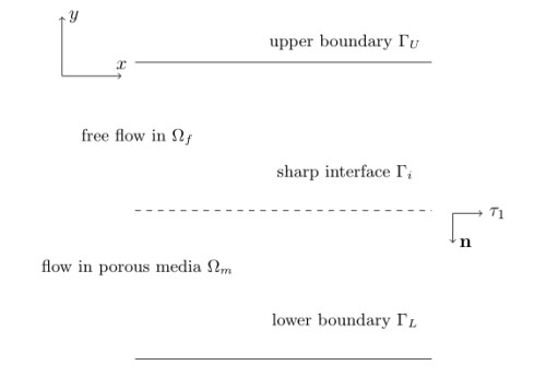
This study investigates the global well-posedness of a coupled Navier–Stokes–Darcy model incorporating the Beavers–Joseph–Saffman–Jones interface boundary condition in two-dimensional Euclidean space. We establish the existence of global strong solutions for the system in both linear and nonlinear cases where porosity depends on pressure. When dealing with the time-dependent porous media, the primary challenge in obtaining closed prior estimates arises from the presence of complex, sharp interfaces. To address this issue, we employ the classical Trace Theorem. Such space-time variable coupled systems are crucial for understanding underground fluid flow.

References

[1]	J. R. Fanchi, Principles of Applied Reservoir Simulation, Elsevier, 2005.
[2]	J. Bear, Dynamics of Fluids in Porous Media, Courier Corporation, 1972.
[3]	H. Knüpfer, N. Masmoudi, Well-posedness and uniform bounds for a nonlocal third order evolution operator on an infinite wedge, Commun. Math. Phys., 320 (2013), 395–424. https://doi.org/10.1007/s00220-013-1708-z doi: 10.1007/s00220-013-1708-z
[4]	D. A. Nield, A. Bejan, Convection in Porous Media, New York: Springer, 1992.
[5]	H. K. Versteeg, W. Malalasekera, The finite volume method, in An Introduction to Computational Fluid Dynamics, Pearson Education, 2007.
[6]	S. Whitaker, Flow in porous media I: A theoretical derivation of Darcy's law, Transp. Porous Media, 1 (1986), 3–25. https://doi.org/10.1007/BF01036523 doi: 10.1007/BF01036523
[7]	L. C. Evans, Measure Theory and Fine Properties of Functions, Routledge, 2018. https://doi.org/10.1201/9780203747940
[8]	A. Çeşmelioğlu, B. Rivière, Analysis of time-dependent Navier-Stokes flow coupled with Darcy flow, J. Numer. Math., 16 (2008), 249–280. https://doi.org/10.1515/JNUM.2008.012 doi: 10.1515/JNUM.2008.012
[9]	A. Çeşmelioğlu, B. Rivière, Primal discontinuous Galerkin methods for time-dependent coupled surface and subsurface flow, J. Sci. Comput., 40 (2009), 115–140. https://doi.org/10.1007/s10915-009-9274-4 doi: 10.1007/s10915-009-9274-4
[10]	P. G. Saffman, On the boundary condition at the surface of a porous medium, Stud. Appl. Math., 50 (1971), 93–101. https://doi.org/10.1002/sapm197150293 doi: 10.1002/sapm197150293
[11]	D. Han, X. He, Q. Wang, Y. Wu, Existence and weak-strong uniqueness of solutions to the Cahn-Hilliard-Navier-Stokes-Darcy system in superposed free flow and porous media, Nonlinear Anal., 211 (2021), 112411. https://doi.org/10.1016/j.na.2021.112411 doi: 10.1016/j.na.2021.112411
[12]	V. Girault, B. Rivière, DG approximation of coupled Navier-Stokes and Darcy equations by Beaver-Joseph-Saffman interface condition, SIAM J. Numer. Anal., 47 (2009), 2052–2089. https://doi.org/10.1137/070686081 doi: 10.1137/070686081
[13]	M. Cai, M. Mu, J. Xu, Numerical solution to a mixed Navier-Stokes/Darcy model by the two-grid approach, SIAM J. Numer. Anal., 47 (2009), 3325–3338. https://doi.org/10.1137/080721868 doi: 10.1137/080721868
[14]	G. Du, L. Zuo, Local and parallel finite element method for the mixed Navier-Stokes/Darcy model with Beavers-Joseph interface conditions, Acta Math. Sci., 37 (2017), 1331–1347. https://doi.org/10.1016/S0252-9602(17)30076-0 doi: 10.1016/S0252-9602(17)30076-0
[15]	C. Qiu, X. He, J. Li, Y. Lin, A domain decomposition method for the time-dependent Navier-Stokes-Darcy model with Beavers-Joseph interface condition and defective boundary condition, J. Comput. Phys., 411 (2020), 109400. https://doi.org/10.1016/j.jcp.2020.109400 doi: 10.1016/j.jcp.2020.109400
[16]	D. Han, D. Sun, X. Wang, Two-phase flows in karstic geometry, Math. Methods Appl. Sci., 37 (2014), 3048–3063. https://doi.org/10.1002/mma.3043 doi: 10.1002/mma.3043
[17]	X. He, J. Li, Y. Lin, J. Ming, A domain decomposition method for the steady-state Navier-Stokes-Darcy model with Beavers-Joseph interface condition, SIAM J. Sci. Comput., 37 (2015), S264–S290. https://doi.org/10.1137/140965776 doi: 10.1137/140965776
[18]	W. Layton, F. Schieweck, I. Yotov, Coupling fluid flow with porous media flow, SIAM J. Numer. Anal., 40 (2003), 2195–2218. https://doi.org/10.1137/S0036142901392766 doi: 10.1137/S0036142901392766
[19]	M. Discacciati, E. Miglio, A. Quarteroni, Mathematical and numerical models for coupling surface and groundwater flows, Appl. Numer. Math., 43 (2002), 57–74. https://doi.org/10.1016/S0168-9274(02)00125-3 doi: 10.1016/S0168-9274(02)00125-3
[20]	B. Rivière, I. Yotov, Locally conservative coupling of Stokes and Darcy flows, SIAM J. Numer. Anal., 42 (2005), 1959–1977. https://doi.org/10.1137/S0036142903427640 doi: 10.1137/S0036142903427640
[21]	M. Discacciati, A. Quarteroni, A. Valli, Robin-Robin domain decomposition methods for the Stokes-Darcy coupling, SIAM J. Numer. Anal., 45 (2007), 1246–1268. https://doi.org/10.1137/06065091X doi: 10.1137/06065091X
[22]	D. Han, Q. Wang, X. Wang, Dynamic transitions and bifurcations for thermal convection in the superposed free flow and porous media, Physica D, 414 (2020), 132687. https://doi.org/10.1016/j.physd.2020.132687 doi: 10.1016/j.physd.2020.132687
[23]	X. Wang, H. Wu, Global weak solutions to the Navier-Stokes-Darcy-Boussinesq system for thermal convection in coupled free and porous media flows, Adv. Differ. Equations, 26 (2021), 1–44. http://doi.org/10.57262/ade/1610420433 doi: 10.57262/ade/1610420433
[24]	Y. Gao, D. Han, X. He, U. Rüde, Unconditionally stable numerical methods for Cahn-Hilliard-Navier-Stokes-Darcy system with different densities and viscosities, J. Comput. Phys., 454 (2022), 110968. https://doi.org/10.1016/j.jcp.2022.110968 doi: 10.1016/j.jcp.2022.110968
[25]	W. Chen, D. Han, X. Wang, Y. Zhang, Uniquely solvable and energy stable decoupled numerical schemes for the Cahn-Hilliard-Navier-Stokes-Darcy-Boussinesq system, J. Sci. Comput., 85 (2020), 45. https://doi.org/10.1007/s10915-020-01341-7 doi: 10.1007/s10915-020-01341-7
[26]	Y. Gao, X. He, L. Mei, X. Yang, Decoupled, linear, and energy stable finite element method for the Cahn-Hilliard-Navier-Stokes-Darcy phase field model, SIAM J. Sci. Comput., 40 (2018), B110–B137. https://doi.org/10.1137/16M1100885 doi: 10.1137/16M1100885
[27]	D. Han, X. Wang, H. Wu, Existence and uniqueness of global weak solutions to a Cahn-Hilliard-Stokes-Darcy system for two phase incompressible flows in karstic geometry, J. Differ. Equations, 257 (2014), 3887–3933. https://doi.org/10.1016/j.jde.2014.07.013 doi: 10.1016/j.jde.2014.07.013
[28]	C. Foias, O. Manley, R. Temam, Attractors for the Bénard problem: existence and physical bounds on their fractal dimension, Nonlinear Anal. Theory Methods Appl., 11 (1987), 939–967. https://doi.org/10.1016/0362-546X(87)90061-7 doi: 10.1016/0362-546X(87)90061-7
[29]	P. Fabrie, Solutions fortes et comportment asymtotique pour un modèle de convection naturelle en milieu poreux, Acta Appl. Math., 7 (1986), 49–77. https://doi.org/10.1007/BF00046977 doi: 10.1007/BF00046977
[30]	H. V. Ly, E. S. Titi, Global Gevrey regularity for the Bénard convection in a porous medium with zero Darcy-Prandtl number, J. Nonlinear Sci., 9 (1999), 333–362. https://doi.org/10.1007/s003329900073 doi: 10.1007/s003329900073
[31]	M. McCurdy, N. Moore, X. Wang, Convection in a coupled free flow-porous media system, SIAM J. Appl. Math., 79 (2019), 2313–2339. https://doi.org/10.1137/19M1238095 doi: 10.1137/19M1238095
[32]	G. S. Beavers, D. D. Joseph, Boundary conditions at a naturally permeable wall, J. Fluid Mech., 30 (1967), 197–207. https://doi.org/10.1017/S0022112067001375 doi: 10.1017/S0022112067001375
[33]	I. P. Jones, Low Reynolds number flow past a porous spherical shell, Math. Proc. Cambridge Philos. Soc., 73 (1973), 231–238. https://doi.org/10.1017/S0305004100047642 doi: 10.1017/S0305004100047642
[34]	H. W. Alt, S. Luckhaus, Quasilinear elliptic-parabolic differential equations, Math. Z., 3 (1983), 311–342.
[35]	P. Fabrie, M. Langlais, Mathematical analysis of miscible displacement in porous medium, SIAM J. Math. Anal., 23 (1992), 1375–1392. https://doi.org/10.1137/0523079 doi: 10.1137/0523079
[36]	P. Fabrie, T. Gallouët, Modelling wells in porous media flows, Math. Models Methods Appl. Sci., 10 (2000), 673–709. https://doi.org/10.1142/S0218202500000367 doi: 10.1142/S0218202500000367
[37]	F. Marpeau, M. Saad, Mathematical analysis of radionuclides displacement in porous media with nonlinear adsorption, J. Differ. Equations, 228 (2006), 412–439. https://doi.org/10.1016/j.jde.2006.03.023 doi: 10.1016/j.jde.2006.03.023
[38]	P. Liu, W. Liu, Global well-posedness of an initial-boundary value problem of the 2-D incompressible Navier-Stokes-Darcy system, Acta Appl. Math., 160 (2019), 101–128. https://doi.org/10.1007/s10440-018-0197-7 doi: 10.1007/s10440-018-0197-7
[39]	M. Cui, W. Dong, Z. Guo, Global well-posedness of coupled Navier-Stokes and Darcy equations, J. Differ. Equations, 388 (2024), 82–111. https://doi.org/10.1016/j.jde.2023.12.044 doi: 10.1016/j.jde.2023.12.044
[40]	L. Tan, M. Cui, B. Cheng, An approach to the global well-posedness of a coupled 3-dimensional Navier-Stokes-Darcy model with Beavers-Joseph-Saffman-Jones interface boundary condition, AIMS Math., 9 (2024), 6993–7016. http://doi.org/10.3934/math.2024341 doi: 10.3934/math.2024341
[41]	A. Çeşmelioğlu, B. Rivière, Existence of a weak solution for the fully coupled Navier-Stokes/Darcy-transport problem, J. Differ. Equations, 252 (2012), 4138–4175. https://doi.org/10.1016/j.jde.2011.12.001 doi: 10.1016/j.jde.2011.12.001
[42]	M. Discacciati, A. Quarteroni, Analysis of a domain decomposition method for the coupling of Stokes and Darcy equations, in Numerical Mathematics and Advanced Applications, Springer Milan, (2003), 3–20. https://doi.org/10.1007/978-88-470-2089-4_1
[43]	A. Çeşmelioğlu, V. Girault, B. Rivière, Time-dependent coupling of Navier-Stokes and Darcy flows, ESAIM. Math. Model. Numer. Anal., 47 (2013), 539–554. https://doi.org/10.1051/m2an/2012034 doi: 10.1051/m2an/2012034
[44]	Y. Hou, D. Xue, Y. Jiang, On the weak solutions to steady-state mixed Navier-Stokes/Darcy model, Acta Math. Sin., 39 (2023), 939–951. https://doi.org/10.1007/s10114-022-9134-9 doi: 10.1007/s10114-022-9134-9
[45]	Z. Chen, G. Huan, Y. Ma, Computational Methods for Multiphase Flows in Porous Media, Society for Industrial and Applied Mathematics, 2006. https://doi.org/10.1137/1.9780898718942
[46]	L. Nirenberg, On elliptic partial differential equations, Ann. Sc. Norm. Super. Pisa Cl. Sci., 13 (1959), 115–162. Available from: http://eudml.org/doc/83226.
[47]	H. Poincaré, Sur les equations aux dérivées partielles de la physique mathématique, Am. J. Math., 12 (1890), 211–294. https://doi.org/10.2307/2369620 doi: 10.2307/2369620
[48]	S. Brenner, Korn's inequalities for piecewise $H^{1}$ vector fields, Math. Comput., 73 (2004), 1067–1087. https://doi.org/10.1090/S0025-5718-03-01579-5 doi: 10.1090/S0025-5718-03-01579-5

Reader Comments

Your name:*

Email:*
© 2024 the Author(s), licensee AIMS Press. This is an open access article distributed under the terms of the Creative Commons Attribution License (http://creativecommons.org/licenses/by/4.0)