Quadrature-free polytopic discontinuous Galerkin methods for transport problems

Thomas J. Radley; Paul Houston; Matthew E. Hubbard; Thomas J. Radley; Paul Houston; Matthew E. Hubbard

doi:10.3934/mine.2024009

Mathematics in Engineering

2024, Volume 6, Issue 1: 192-220. doi: 10.3934/mine.2024009

Previous Article Next Article

Research article Special Issues

Quadrature-free polytopic discontinuous Galerkin methods for transport problems

School of Mathematical Sciences, University of Nottingham, University Park, Nottingham NG7 2RD, UK

Received: 30 July 2023 Revised: 15 December 2023 Accepted: 14 February 2024 Published: 05 March 2024

In this article we consider the application of Euler's homogeneous function theorem together with Stokes' theorem to exactly integrate families of polynomial spaces over general polygonal and polyhedral (polytopic) domains in two and three dimensions, respectively. This approach allows for the integrals to be evaluated based on only computing the values of the integrand and its derivatives at the vertices of the polytopic domain, without the need to construct a sub-tessellation of the underlying domain of interest. Here, we present a detailed analysis of the computational complexity of the proposed algorithm and show that this depends on three key factors: the ambient dimension of the underlying polytopic domain; the size of the requested polynomial space to be integrated; and the size of a directed graph related to the polytopic domain. This general approach is then employed to compute the volume integrals arising within the discontinuous Galerkin finite element approximation of the linear transport equation. Numerical experiments are presented which highlight the efficiency of the proposed algorithm when compared to standard quadrature approaches defined on a sub-tessellation of the polytopic elements.
- polytopic elements,
- numerical integration,
- discontinuous Galerkin methods
Citation: Thomas J. Radley, Paul Houston, Matthew E. Hubbard. Quadrature-free polytopic discontinuous Galerkin methods for transport problems[J]. Mathematics in Engineering, 2024, 6(1): 192-220. doi: 10.3934/mine.2024009

Related Papers:

Abstract

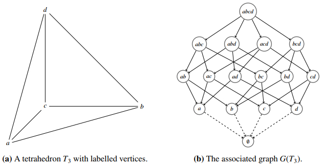
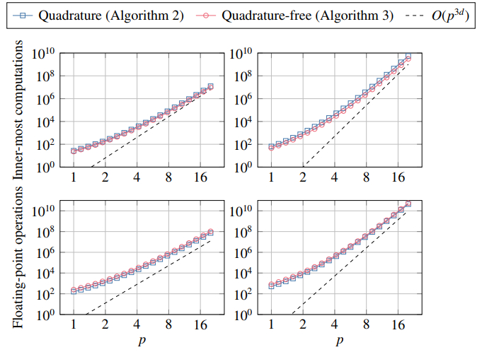
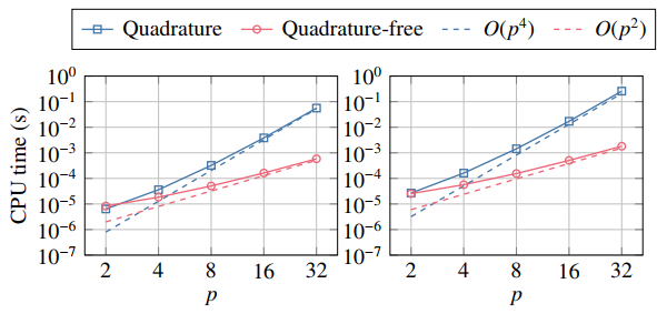
In this article we consider the application of Euler's homogeneous function theorem together with Stokes' theorem to exactly integrate families of polynomial spaces over general polygonal and polyhedral (polytopic) domains in two and three dimensions, respectively. This approach allows for the integrals to be evaluated based on only computing the values of the integrand and its derivatives at the vertices of the polytopic domain, without the need to construct a sub-tessellation of the underlying domain of interest. Here, we present a detailed analysis of the computational complexity of the proposed algorithm and show that this depends on three key factors: the ambient dimension of the underlying polytopic domain; the size of the requested polynomial space to be integrated; and the size of a directed graph related to the polytopic domain. This general approach is then employed to compute the volume integrals arising within the discontinuous Galerkin finite element approximation of the linear transport equation. Numerical experiments are presented which highlight the efficiency of the proposed algorithm when compared to standard quadrature approaches defined on a sub-tessellation of the polytopic elements.

References

[1]	P. F. Antonietti, A. Cangiani, J. Collis, Z. Dong, E. H. Georgoulis, S. Giani, et al., Review of discontinuous Galerkin finite element methods for partial differential equations on complicated domains, In: G. R. Barrenechea, F. Brezzi, A. Cangiani, E. H. Georgoulis, Building bridges: connections and challenges in modern approaches to numerical partial differential equations, Cham: Springer, 114 (2016), 281–310. https://doi.org/10.1007/978-3-319-41640-3_9
[2]	P. F. Antonietti, P. Houston, G. Pennesi, Fast numerical integration on polytopic meshes with applications to discontinuous Galerkin finite element methods, J. Sci. Comput., 77 (2018), 1339–1370. https://doi.org/10.1007/s10915-018-0802-y doi: 10.1007/s10915-018-0802-y
[3]	L. Beirão Da Veiga, F. Brezzi, A. Cangiani, G. Manzini, L. D. Marini, A. Russo, Basic principles of virtual element methods, Math. Models Methods Appl. Sci., 23 (2013), 199–214. https://doi.org/10.1142/S0218202512500492 doi: 10.1142/S0218202512500492
[4]	B. Büeler, A. Enge, K. Fukuda, Exact volume computation for polytopes: a practical study, In: G. Kalai, G. M. Ziegler, Polytopes–Combinatorics and computation, DMV Seminar, Basel: Birkhäuser, 29 (2000), 131–154. https://doi.org/10.1007/978-3-0348-8438-9_6
[5]	A. Cangiani, Z. Dong, E. H. Georgoulis, P. Houston, $hp$-version discontinuous Galerkin methods on polygonal and polyhedral meshes, Cham: Springer, 2017. https://doi.org/10.1007/978-3-319-67673-9
[6]	A. Cangiani, E. H. Georgoulis, P. Houston, hp-version discontinuous Galerkin methods on polygonal and polyhedral meshes, Math. Models Methods Appl. Sci., 24 (2014), 2009–2041. https://doi.org/10.1142/S0218202514500146 doi: 10.1142/S0218202514500146
[7]	E. B. Chin, J. B. Lasserre, N. Sukumar, Numerical integration of homogeneous functions on convex and nonconvex polygons and polyhedra, Comp. Mech., 56 (2015), 967–981. https://doi.org/10.1007/s00466-015-1213-7 doi: 10.1007/s00466-015-1213-7
[8]	E. B. Chin, N. Sukumar, An efficient method to integrate polynomials over polytopes and curved solids, Comput. Aided Geom. Design, 82 (2020), 101914. https://doi.org/10.1016/j.cagd.2020.101914 doi: 10.1016/j.cagd.2020.101914
[9]	M. Cicuttin, A. Ern, N. Pignet, Hybrid high-order methods: a primer with applications to solid mechanics, Cham: Springer, 2021. https://doi.org/10.1007/978-3-030-81477-9
[10]	Z. Dong, E. H. Georgoulis, T. Kappas, GPU-accelerated discontinuous Galerkin methods on polytopic meshes, SIAM J. Sci. Comput., 43 (2021), C312–C334. https://doi.org/10.1137/20M1350984 doi: 10.1137/20M1350984
[11]	M. G. Duffy, Quadrature over a pyramid or cube of integrands with a singularity at a vertex, SIAM J. Numer. Anal., 19 (1982), 1260–1262. https://doi.org/10.1137/0719090 doi: 10.1137/0719090
[12]	B. Grünbaum, V. Klee, M. A. Perles, G. C. Shephard, Convex polytopes, Vol. 16, 1 Ed., New York: Interscience, 1967.
[13]	P. Houston, M. E. Hubbard, T. J. Radley, O. J. Sutton, R. S. J. Widdowson, Efficient high-order space-angle-energy polytopic discontinuous Galerkin finite element methods for linear Boltzmann transport, arXiv, 2023. https://doi.org/10.48550/arXiv.2304.09592
[14]	V. Kaibel, M. E. Pfetsch, Computing the face lattice of a polytope from its vertex-facet incidences, Comp. Geom., 23 (2002), 281–290. https://doi.org/10.1016/S0925-7721(02)00103-7 doi: 10.1016/S0925-7721(02)00103-7
[15]	G. Karypis, V. Kumar, A fast and highly quality multilevel scheme for partitioning irregular graphs, SIAM J. Sci. Comput., 20 (1998), 359–392. https://doi.org/10.1137/S1064827595287997 doi: 10.1137/S1064827595287997
[16]	D. E. Knuth, The art of computer programming, Vol. 2, Seminumerical Algorithms, 3 Eds., Addison-Wesley, 1981.
[17]	J. Lasserre, Integration on a convex polytope, Proc. Amer. Math. Soc., 126 (1998), 2433–2441.
[18]	J. B. Lasserre, Integration and homogeneous functions, Proc. Amer. Math. Soc., 127 (1999), 813–818.
[19]	J. N. Lyness, G. Monegato, Quadrature rules for regions having regular hexagonal symmetry, SIAM J. Numer. Anal., 14 (1977), 283–295. https://doi.org/10.1137/0714018 doi: 10.1137/0714018
[20]	S. E. Mousavi, H. Xiao, N. Sukumar, Generalized Gaussian quadrature rules on arbitrary polygons, Int. J. Numer. Methods Eng., 82 (2010), 99–113. https://doi.org/10.1002/nme.2759 doi: 10.1002/nme.2759
[21]	S. E. Mousavi, N. Sukumar, Numerical integration of polynomials and discontinuous functions on irregular convex polygons and polyhedrons, Comput. Mech., 47 (2011), 535–554. https://doi.org/10.1007/s00466-010-0562-5 doi: 10.1007/s00466-010-0562-5
[22]	C. P. Simon, L. Blume, Mathematics for economists, Vol. 7, New York: Norton, 1994.
[23]	A. Stroud, Approximate calculation of multiple integrals, Prentice-Hall series in automatic computation, Prentice-Hall, Inc., 1971.
[24]	Y. Sudhakar, W. A. Wall, Quadrature schemes for arbitrary convex/concave volumes and integration of weak form in enriched partition of unity methods, Comput. Methods Appl. Mech. Eng., 258 (2013), 39–54. https://doi.org/10.1016/j.cma.2013.01.007 doi: 10.1016/j.cma.2013.01.007
[25]	N. Sukumar, A. Tabarraei, Conforming polygonal finite elements, Int. J. Numer. Methods Eng., 61 (2004), 2045–2066. https://doi.org/10.1002/nme.1141 doi: 10.1002/nme.1141
[26]	M. E. Taylor, Partial differential equations: basic theory, Vol. 1, Springer, 1996.
[27]	H. Xiao, Z. Gimbutas, A numerical algorithm for the construction of efficient quadrature rules in two and higher dimensions, Comput. Math. Appl., 59 (2010), 663–676. https://doi.org/10.1016/j.camwa.2009.10.027 doi: 10.1016/j.camwa.2009.10.027

Reader Comments

Your name:*

Email:*
© 2024 the Author(s), licensee AIMS Press. This is an open access article distributed under the terms of the Creative Commons Attribution License (http://creativecommons.org/licenses/by/4.0)