Five genes involved in circular RNA-associated competitive endogenous RNA network correlates with metastasis in papillary thyroid carcinoma

Jie Qiu; Maolin Sun; Chuanshan Zang; Liwei Jiang; Zuorong Qin; Yan Sun; Mingbo Liu; Wenwei Zhang; Jie Qiu; Maolin Sun; Chuanshan Zang; Liwei Jiang; Zuorong Qin; Yan Sun; Mingbo Liu; Wenwei Zhang

doi:10.3934/mbe.2021444

Mathematical Biosciences and Engineering

2021, Volume 18, Issue 6: 9016-9032. doi: 10.3934/mbe.2021444

Previous Article Next Article

Research article

Five genes involved in circular RNA-associated competitive endogenous RNA network correlates with metastasis in papillary thyroid carcinoma

1.
Department of Otolaryngology, The Affiliated Hospital of Qingdao University, Qingdao 266003, China
2.
Department of Otolaryngology, Hainan Hospital of PLA General Hospital, Sanya 572000, China
3.
Radiology Department, The Affiliated Hospital of Qingdao University, Qingdao 266003, China
† These authors contributed equally to this work

Received: 30 July 2021 Accepted: 27 September 2021 Published: 21 October 2021

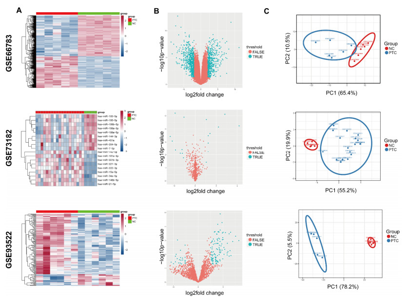
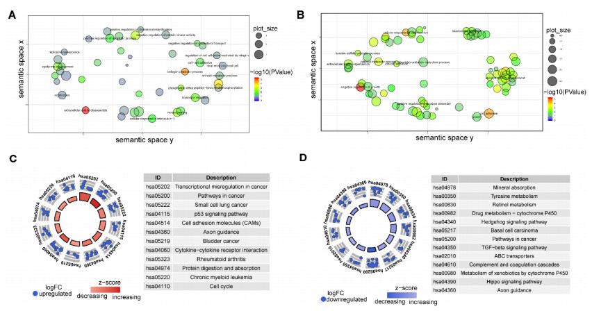
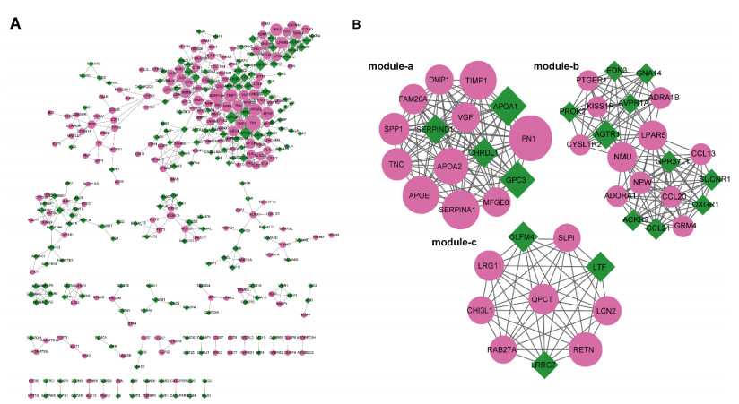
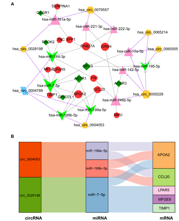
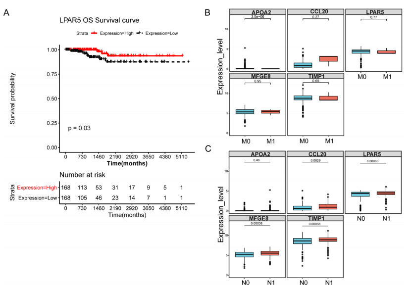
This study aimed to identify potential circular RNA (circRNA), microRNA (miRNA) and mRNA biomarkers as well as their underlying regulatory mechanisms in papillary thyroid carcinoma (PTC). Three microarray datasets from the Gene Expression Omnibus database as well as expression data and clinical phenotype from The Cancer Genome Atlas (TCGA) were downloaded, followed by differential expression, functional enrichment, protein–protein interaction (PPI), and module analyses. The support vector machine (SVM)-recursive feature elimination (RFE) algorithm was used to screen the key circRNAs. Finally, the mRNA-miRNA-circRNA regulatory network and competitive endogenous RNA (ceRNA) network were constructed. The prognostic value and clinical correlations of key mRNAs were investigated using TCGA dataset, and their expression was validated using the UALCAN database. A total of 1039 mRNAs, 18 miRNAs and 137 circRNAs were differentially expressed in patients with PTC. A total of 37 key circRNAs were obtained using the SVM-RFE algorithm, whereas 46 key mRNAs were obtained from significant modules in the PPI network. A total of 11 circRNA-miRNA pairs and 40 miRNA-mRNA pairs were predicted. Based on these interaction pairs, 46 circRNA-miRNA-mRNA regulatory pairs were integrated, of which 8 regulatory pairs in line with the ceRNA hypothesis were obtained, including two circRNAs (circ_0004053 and circ_0028198), three miRNAs (miR-199a-5p, miR-199b-5p, and miR-7-5p), and five mRNAs, namely APOA2, CCL20, LPAR5, MFGE8, and TIMP1. Survival analysis showed that LPAR5 expression was associated with patient survival. APOA2 expression showed significant differences between metastatic and non-metastatic tumors, whereas CCL20, LPAR5, MFGE8 and TIMP1 showed significant differences between metastatic and non-metastatic lymph nodes. Overall, we identified several potential targets and regulatory mechanisms involved in PTC. APOA2, CCL20, LPAR5, MFGE8, and TIMP1 may be correlated with PTC metastasis.
- papillary thyroid carcinoma,
- circular RNAs,
- ceRNA,
- metastasis
Citation: Jie Qiu, Maolin Sun, Chuanshan Zang, Liwei Jiang, Zuorong Qin, Yan Sun, Mingbo Liu, Wenwei Zhang. Five genes involved in circular RNA-associated competitive endogenous RNA network correlates with metastasis in papillary thyroid carcinoma[J]. Mathematical Biosciences and Engineering, 2021, 18(6): 9016-9032. doi: 10.3934/mbe.2021444

Related Papers:

Abstract

This study aimed to identify potential circular RNA (circRNA), microRNA (miRNA) and mRNA biomarkers as well as their underlying regulatory mechanisms in papillary thyroid carcinoma (PTC). Three microarray datasets from the Gene Expression Omnibus database as well as expression data and clinical phenotype from The Cancer Genome Atlas (TCGA) were downloaded, followed by differential expression, functional enrichment, protein–protein interaction (PPI), and module analyses. The support vector machine (SVM)-recursive feature elimination (RFE) algorithm was used to screen the key circRNAs. Finally, the mRNA-miRNA-circRNA regulatory network and competitive endogenous RNA (ceRNA) network were constructed. The prognostic value and clinical correlations of key mRNAs were investigated using TCGA dataset, and their expression was validated using the UALCAN database. A total of 1039 mRNAs, 18 miRNAs and 137 circRNAs were differentially expressed in patients with PTC. A total of 37 key circRNAs were obtained using the SVM-RFE algorithm, whereas 46 key mRNAs were obtained from significant modules in the PPI network. A total of 11 circRNA-miRNA pairs and 40 miRNA-mRNA pairs were predicted. Based on these interaction pairs, 46 circRNA-miRNA-mRNA regulatory pairs were integrated, of which 8 regulatory pairs in line with the ceRNA hypothesis were obtained, including two circRNAs (circ_0004053 and circ_0028198), three miRNAs (miR-199a-5p, miR-199b-5p, and miR-7-5p), and five mRNAs, namely APOA2, CCL20, LPAR5, MFGE8, and TIMP1. Survival analysis showed that LPAR5 expression was associated with patient survival. APOA2 expression showed significant differences between metastatic and non-metastatic tumors, whereas CCL20, LPAR5, MFGE8 and TIMP1 showed significant differences between metastatic and non-metastatic lymph nodes. Overall, we identified several potential targets and regulatory mechanisms involved in PTC. APOA2, CCL20, LPAR5, MFGE8, and TIMP1 may be correlated with PTC metastasis.

References

[1]	B. Jankovic, K. T. Le, J. M. Hershman, Hashimoto's thyroiditis and papillary thyroid carcinoma: is there a correlation?, J. Clin. Endocrinol. Metab., 98 (2013), 474-482. doi: 10.1210/jc.2012-2978
[2]	D. S. McLeod, A. M. Sawka, D. S. Cooper, Controversies in primary treatment of low-risk papillary thyroid cancer, The Lancet, 381 (2013), 1046-1057. doi: 10.1016/S0140-6736(12)62205-3
[3]	A. Cummings, M. Goldfarb, Thyroid carcinoma metastases to axillary lymph nodes: report of two rare cases of papillary and medullary thyroid carcinoma and literature review, Endocr. Pract., 20 (2014), e34-e37. doi: 10.4158/EP13339.CR
[4]	G. H. Sakorafas, D. Sampanis, M. Safioleas, Cervical lymph node dissection in papillary thyroid cancer: current trends, persisting controversies, and unclarified uncertainties, Surg. Oncol., 19 (2010), e57-e70. doi: 10.1016/j.suronc.2009.04.002
[5]	L. L. Chen, The biogenesis and emerging roles of circular RNAs, Nat. Rev. Mol. Cell Bio., 17 (2016), 205-211. doi: 10.1038/nrm.2015.32
[6]	H. L. Sanger, G. Klotz, D. Riesner, H. J. Gross, A. K. Kleinschmidt, Viroids are single-stranded covalently closed circular RNA molecules existing as highly base-paired rod-like structures, Proc. Natl. Acad. Sci., 73 (1976), 3852-3856. doi: 10.1073/pnas.73.11.3852
[7]	J. Li, J. Yang, P. Zhou, Y. Le, C. Zhou, S. Wang, et al., Circular RNAs in cancer: novel insights into origins, properties, functions and implications, Am. J. Cancer Res., 5 (2015), 472-480.
[8]	Y. Zhang, X. O. Zhang, T. Chen, J. F. Xiang, Q. F. Yin, Y. H. Xing, et al., Circular intronic long noncoding RNAs, Mol. Cell, 51 (2013), 792-806. doi: 10.1016/j.molcel.2013.08.017
[9]	W. R. Jeck, N. E. Sharpless, Detecting and characterizing circular RNAs, Nat. Biotechnol., 32 (2014), 453-461. doi: 10.1038/nbt.2890
[10]	Z. Zhong, M. Huang, M. Lv, Y. He, C. Duan, L. Zhang, et al., Circular RNA MYLK as a competing endogenous RNA promotes bladder cancer progression through modulating VEGFA/VEGFR2 signaling pathway, Cancer Lett., 403 (2017), 305-317. doi: 10.1016/j.canlet.2017.06.027
[11]	L. Lü, J. Sun, P. Shi, W. Kong, K. Xu, B. He, et al., Identification of circular RNAs as a promising new class of diagnostic biomarkers for human breast cancer, Oncotarget, 8 (2017), 44096-44107. doi: 10.18632/oncotarget.17307
[12]	K. Y. Hsiao, Y. C. Lin, S. K. Gupta, N. Chang, L. Yen, H. S. Sun, et al., Noncoding effects of circular RNA CCDC66 promote colon cancer growth and metastasis, Cancer Res., 77 (2017), 2339-2350. doi: 10.1158/0008-5472.CAN-16-1883
[13]	D. Han, J. Li, H. Wang, X. Su, J. Hou, Y. Gu, et al., Circular RNA circMTO1 acts as the sponge of microRNA-9 to suppress hepatocellular carcinoma progression, Hepatology, 66 (2017), 1151-1164. doi: 10.1002/hep.29270
[14]	G. K. Smyth, LIMMA: linear models for microarray data, in Bioinformatics and Computational Biology Solutions Using R and Bioconductor, Spring, (2005), 397-420.
[15]	M. Ashburner, C. A. Ball, J. A. Blake, D. Botstein, H. Butler, J. M. Cherry, et al., Gene ontology: tool for the unification of biology, Nat. Genet., 25 (2000), 25-29. doi: 10.1038/75556
[16]	M. Kanehisa, S. Goto, KEGG: kyoto encyclopedia of genes and genomes, Nucleic Acids Res., 28 (2000), 27-30. doi: 10.1093/nar/28.1.27
[17]	D. Szklarczyk, A. Franceschini, S. Wyder, K. Forslund, D. Heller, J. Huerta-Cepas, et al., STRING v10: protein–protein interaction networks, integrated over the tree of life, Nucleic Acids Res., 43 (2015), D447-D452. doi: 10.1093/nar/gku1003
[18]	P. Shannon, A. Markiel, O. Ozier, N. S. Baliga, J. T. Wang, D. Ramage, et al., Cytoscape: a software environment for integrated models of biomolecular interaction networks, Genome Research, 13 (2003), 2498-2504. doi: 10.1101/gr.1239303
[19]	W. P. Bandettini, P. Kellman, C. Mancini, O. J. Booker, S. Vasu, S. W. Leung, et al., MultiContrast delayed enhancement (MCODE) improves detection of subendocardial myocardial infarction by late gadolinium enhancement cardiovascular magnetic resonance: a clinical validation study, J. Cardiovasc. Magn. Reson., 14 (2012), 83. doi: 10.1186/1532-429X-14-83
[20]	H. D. Zhang, L. H. Jiang, D. W. Sun, J. C. Hou, Z. L. Ji, et al., CircRNA: a novel type of biomarker for cancer, Breast Cancer, 25 (2018), 1-7. doi: 10.1007/s12282-017-0793-9
[21]	G. Wu, W. Zhou, X. Pan, Z. Sun, Y. Sun, H. Xu, et al., Circular RNA profiling reveals exosomal circ_0006156 as a novel biomarker in papillary thyroid cancer, Mol. Ther. Nucleic. Acids, 19 (2020), 1134-1144. doi: 10.1016/j.omtn.2019.12.025
[22]	Q. Liu, L. Z. Pan, M. Hu, J. Y. Ma, Molecular network-based identification of circular RNA-associated cerna network in papillary thyroid cancer, Pathol. Oncol. Res., 26 (2020), 1293-1299. doi: 10.1007/s12253-019-00697-y
[23]	S. Borran, G. Ahmadi, S. Rezaei, M. M. Anari, M. Modabberi, Z. Azarash, et al., Circular RNAs: new players in thyroid cancer, Pathol. Res. Pract., 216 (2020), 153217. doi: 10.1016/j.prp.2020.153217
[24]	X. Li, J. Ding, X. Wang, Z. Cheng, Q. Zhu, NUDT21 regulates circRNA cyclization and ceRNA crosstalk in hepatocellular carcinoma, Oncogene, 39 (2020), 891-904. doi: 10.1038/s41388-019-1030-0
[25]	P. F. Tussy, I. R. Maldonado, C. F. Hernando, MicroRNAs and circular RNAs in lipoprotein metabolism, Curr. Atheroscler. Rep., 23 (2021), 33. doi: 10.1007/s11883-021-00934-3
[26]	G. Yu, Z. Yang, T. Peng, Y. Lv, Circular RNAs: rising stars in lipid metabolism and lipid disorders, J. Cell Physiol., 236 (2021), 4797-4806. doi: 10.1002/jcp.30200
[27]	L. Wang, Z. Zheng, X. Feng, X. Zang, W. Ding, F. Wu, et al., circRNA/lncRNA-miRNA-mRNA network in oxidized, low-density, lipoprotein-induced foam cells, DNA Cell Biol., 38 (2019), 1499-1511. doi: 10.1089/dna.2019.4865
[28]	H. Y. Zhang, C. H. Li, X. C. Wang, Y. Q.Luo, X. D. Cao, J. J. Chen, MiR-199 inhibits EMT and invasion of hepatoma cells through inhibition of Snail expression, Eur. Rev. Med. Pharmacol. Sci., 23 (2019), 7884-7891.
[29]	K. Koshizuka, T. Hanazawa, N. Kikkawa, T. Arai, A. Okato, A. Kurozumi, et al., Regulation of ITGA3 by the anti-tumor miR-199 family inhibits cancer cell migration and invasion in head and neck cancer, Cancer Sci., 108 (2017), 1681-1692. doi: 10.1111/cas.13298
[30]	T. B. Hansen, J. Kjems, C. K. Damgaard, Circular RNA and miR-7 in cancer, Cancer Res., 73 (2013), 5609-5612. doi: 10.1158/0008-5472.CAN-13-1568
[31]	H. Xiao, MiR-7-5p suppresses tumor metastasis of non-small cell lung cancer by targeting NOVA2, Cell Mol. Biol. Lett., 24 (2019), 60. doi: 10.1186/s11658-019-0188-3
[32]	K. Zeng, X. Chen, M. Xu, X. Liu, X. Hu, T. Xu, et al., CircHIPK3 promotes colorectal cancer growth and metastasis by sponging miR-7, Cell Death Dis., 9 (2018), 417. doi: 10.1038/s41419-018-0454-8
[33]	T. Hong, J. Ding, W. Li, miR-7 reverses breast cancer resistance to chemotherapy by targeting MRP1 and BCL2, Onco. Targets Ther., 12 (2019), 11097-11105. doi: 10.2147/OTT.S213780
[34]	J. Xia, T. Cao, C. Ma, Y. Shi, Y. Sun, Z. P. Wang, et al., MiR-7 suppresses tumor progression by directly targeting MAP3K9 in pancreatic cancer, Mol. Ther. Nucleic Acids, 13 (2018), 121-132. doi: 10.1016/j.omtn.2018.08.012
[35]	W. Shi, J. Song, Z. Gao, X. Liu, W. Wang, Downregulation of miR-7-5p Inhibits the Tumorigenesis of esophagus cancer via Targeting KLF4, Onco. Targets Ther., 13 (2020), 9443-9453. doi: 10.2147/OTT.S251508
[36]	Y. Duan, Y. Zhang, W. Peng, P. Jiang, Z. Deng, C. Wu, MiR-7-5pand miR-451 as diagnostic biomarkers for papillary thyroid carcinoma in formalin-fixed paraffin-embedded tissues, Pharmazie, 75 (2020), 266-270.
[37]	J. Y. Han, S. Guo, N. Wei, R. Xue, W. Li, G. Dong, et al, CiRS-7 promotes the proliferation and migration of papillary thyroid cancer by negatively regulating the miR-7/epidermal growth factor receptor axis, Biomed Res. Int., 2020 (2020), 9875636.
[38]	K. Honda, V. A. Katzke, A. Hüsing, S. Okaya, H. Shoji, K. Onidani, et al., CA19-9 and apolipoprotein-A2 isoforms as detection markers for pancreatic cancer: a prospective evaluation, Int. J. Cancer, 144 (2019), 1877-1887. doi: 10.1002/ijc.31900
[39]	Y. Sato, T. Kobayashi, S. Nishiumi, A. Okada, T. Fujita, T. Sanuki, et al., Prospective study using plasma apolipoprotein a2-isoforms to screen for high-risk status of pancreatic cancer, Cancers (Basel), 12 (2020), 2625. doi: 10.3390/cancers12092625
[40]	W. Zeng, H. Chang, M. Ma, Y. Li, CCL20/CCR6 promotes the invasion and migration of thyroid cancer cells via NF-kappa B signaling-induced MMP-3 production, Exp Mol. Pathol., 97 (2014), 184-190. doi: 10.1016/j.yexmp.2014.06.012
[41]	C. Y. Wu, C. Zheng, E. J. Xia, R. Quan, J. Hu, X. Zhang, et al., Lysophosphatidic acid receptor 5 (LPAR5) plays a significance role in papillary thyroid cancer via phosphatidylinositol 3-Kinase/Akt/Mammalian target of rapamycin (mTOR) pathway, Med. Sci. Monit., 26 (2020), e919820.
[42]	W. J. Zhao, L. L. Zhu, W. Q. Yang, S. J. Xu, J. Chen, X. F. Ding, et al., LPAR5 promotes thyroid carcinoma cell proliferation and migration by activating class IA PI3K catalytic subunit p110β, Cancer Sci., 112 (2021), 1624-1632. doi: 10.1111/cas.14837
[43]	L. Yu, R. Hu, C. Sullivan, R J. Swanson, S. Oehninger, Y. P. Sun, et al., MFGE8 regulates TGF-β-induced epithelial mesenchymal transition in endometrial epithelial cells in vitro, Reproduction, 152 (2016), 225-233.
[44]	B. Wang, Z. Ge, Y. Wu, Y. Zha, X. Zhang, Y. Yan, et al., MFGE8 is down-regulated in cardiac fibrosis and attenuates endothelial-mesenchymal transition through Smad2/3-Snail signalling pathway, J. Cell. Mol. Med., 24 (2020), 12799-12812. doi: 10.1111/jcmm.15871
[45]	H. W. Jackson, V. Defamie, P. Waterhouse, R. Khokha, TIMPs: versatile extracellular regulators in cancer, Nat. Rev. Cancer, 17 (2017), 38-53. doi: 10.1038/nrc.2016.115
[46]	W. Q. Zhang, W. Sun, Y. Qin, C. Wu, L. He, T. Zhang, et al., Knockdown of KDM1A suppresses tumour migration and invasion by epigenetically regulating the TIMP1/MMP9 pathway in papillary thyroid cancer, J. Cell. Mol. Med., 23 (2019), 4933-4944. doi: 10.1111/jcmm.14311

mbe-18-06-444 supplement.docx

Reader Comments

Your name:*

Email:*
© 2021 the Author(s), licensee AIMS Press. This is an open access article distributed under the terms of the Creative Commons Attribution License (http://creativecommons.org/licenses/by/4.0)