Multi-strategy self-learning particle swarm optimization algorithm based on reinforcement learning

Xiaoding Meng; Hecheng Li; Anshan Chen; Xiaoding Meng; Hecheng Li; Anshan Chen

doi:10.3934/mbe.2023373

Mathematical Biosciences and Engineering

2023, Volume 20, Issue 5: 8498-8530. doi: 10.3934/mbe.2023373

Previous Article Next Article

Research article Special Issues

Multi-strategy self-learning particle swarm optimization algorithm based on reinforcement learning

1.
School of Computer Science and Technology, Qinghai Normal University, Xining 810008, China
2.
School of Mathematics and Statistics, Qinghai Normal University, Xining 810008, China
3.
Academy of Plateau Science and Sustainability, Xining 810008, China

Academic Editor: Yiu-ming Cheung

Received: 19 January 2023 Revised: 15 February 2023 Accepted: 21 February 2023 Published: 03 March 2023

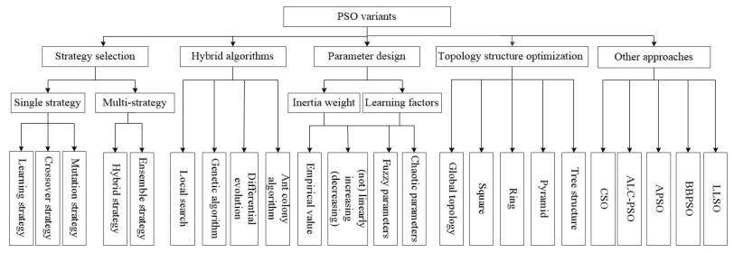
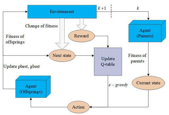
The trade-off between exploitation and exploration is a dilemma inherent to particle swarm optimization (PSO) algorithms. Therefore, a growing body of PSO variants is devoted to solving the balance between the two. Among them, the method of self-adaptive multi-strategy selection plays a crucial role in improving the performance of PSO algorithms but has yet to be well exploited. In this research, with the aid of the reinforcement learning technique to guide the generation of offspring, a novel self-adaptive multi-strategy selection mechanism is designed, and then a multi-strategy self-learning PSO algorithm based on reinforcement learning (MPSORL) is proposed. First, the fitness value of particles is regarded as a set of states that are divided into several state subsets non-uniformly. Second, the $\varepsilon$ -greedy strategy is employed to select the optimal strategy for each particle. The personal best particle and the global best particle are then updated after executing the strategy. Subsequently, the next state is determined. Thus, the value of the Q-table, as a scheme adopted in self-learning, is reshaped by the reward value, the action and the state in a non-stationary environment. Finally, the proposed algorithm is compared with other state-of-the-art algorithms on two well-known benchmark suites and a real-world problem. Extensive experiments indicate that MPSORL has better performance in terms of accuracy, convergence speed and non-parametric tests in most cases. The multi-strategy selection mechanism presented in the manuscript is effective.

Keywords:

Citation: Xiaoding Meng, Hecheng Li, Anshan Chen. Multi-strategy self-learning particle swarm optimization algorithm based on reinforcement learning[J]. Mathematical Biosciences and Engineering, 2023, 20(5): 8498-8530. doi: 10.3934/mbe.2023373

Related Papers:

[1]	Shangbo Zhou, Yuxiao Han, Long Sha, Shufang Zhu . A multi-sample particle swarm optimization algorithm based on electric field force. Mathematical Biosciences and Engineering, 2021, 18(6): 7464-7489. doi: 10.3934/mbe.2021369
[2]	Xin Zhou, Shangbo Zhou, Yuxiao Han, Shufang Zhu . Lévy flight-based inverse adaptive comprehensive learning particle swarm optimization. Mathematical Biosciences and Engineering, 2022, 19(5): 5241-5268. doi: 10.3934/mbe.2022246
[3]	Yufeng Wang, BoCheng Wang, Zhuang Li, Chunyu Xu . A novel particle swarm optimization based on hybrid-learning model. Mathematical Biosciences and Engineering, 2023, 20(4): 7056-7087. doi: 10.3934/mbe.2023305
[4]	Fei Chen, Yanmin Liu, Jie Yang, Meilan Yang, Qian Zhang, Jun Liu . Multi-objective particle swarm optimization with reverse multi-leaders. Mathematical Biosciences and Engineering, 2023, 20(7): 11732-11762. doi: 10.3934/mbe.2023522
[5]	Dongning Chen, Jianchang Liu, Chengyu Yao, Ziwei Zhang, Xinwei Du . Multi-strategy improved salp swarm algorithm and its application in reliability optimization. Mathematical Biosciences and Engineering, 2022, 19(5): 5269-5292. doi: 10.3934/mbe.2022247
[6]	Zhiyan Xing, Yanlong Yang, Zuopeng Hu . Nash equilibrium realization of population games based on social learning processes. Mathematical Biosciences and Engineering, 2023, 20(9): 17116-17137. doi: 10.3934/mbe.2023763
[7]	Qing Wu, Chunjiang Zhang, Mengya Zhang, Fajun Yang, Liang Gao . A modified comprehensive learning particle swarm optimizer and its application in cylindricity error evaluation problem. Mathematical Biosciences and Engineering, 2019, 16(3): 1190-1209. doi: 10.3934/mbe.2019057
[8]	Kefeng Fan, Cun Xu, Xuguang Cao, Kaijie Jiao, Wei Mo . Tri-branch feature pyramid network based on federated particle swarm optimization for polyp segmentation. Mathematical Biosciences and Engineering, 2024, 21(1): 1610-1624. doi: 10.3934/mbe.2024070
[9]	Xuepeng Zheng, Bin Nie, Jiandong Chen, Yuwen Du, Yuchao Zhang, Haike Jin . An improved particle swarm optimization combined with double-chaos search. Mathematical Biosciences and Engineering, 2023, 20(9): 15737-15764. doi: 10.3934/mbe.2023701
[10]	Ruiping Yuan, Jiangtao Dou, Juntao Li, Wei Wang, Yingfan Jiang . Multi-robot task allocation in e-commerce RMFS based on deep reinforcement learning. Mathematical Biosciences and Engineering, 2023, 20(2): 1903-1918. doi: 10.3934/mbe.2023087

Abstract

1. Introduction

With the advancement of computational intelligence technology, many different types of metaheuristic algorithms have emerged. The metaheuristic algorithms can be classified into individual-based metaheuristic algorithms and population-based metaheuristic algorithms. The particle swarm optimization (PSO) algorithm is a representative of population-based intelligence algorithms. PSO is widely used due to its advantages of convergence speed, simplicity and few parameters ^[1]. The application of PSO appeared in various fields ^[2,3,4,5]. However, traditional PSO algorithms have difficulty escaping from the local optimum, resulting in low convergence accuracy. Therefore, lots of improved versions of PSO algorithms have blossomed. Specifically, these PSO variants can be roughly divided into five kinds: 1) strategy selection ^[6,7,8], 2) hybrid algorithms ^[9,10,11], 3) parameter design ^[12,13], 4) topology structure optimization ^[14,15] and 5) other approaches ^{[16,17,18,19,20]}, as shown in Figure 1. Drawing upon five strands of research into PSO variants, this study attempts to further carry out research on the first aspect, i.e., the influence of multi-strategy selection on the performance of PSO.

Figure 1. Classification of PSO variants. (Note that CSO, ALC_PSO, APSO, BBPSO, LLSO are the names of the algorithms proposed in references [16,17,18,19,20].).

DownLoad: Full-Size Img PowerPoint

As briefly reviewed above, a considerable amount of literature has grown up around the theme of a single strategy, such as the learning strategy, the crossover strategy, the mutation strategy and so on. In terms of learning strategies, Liang et al. ^[6] proposed a comprehensive learning PSO algorithm (CLPSO), in which the particles could learn from better particles on the same dimension to increase diversity. CLPSO shows good performance for solving multi-modal optimization problems. Similarly, HCLPSO ^[7] was proposed based on the comprehensive learning (CL) strategy through two-population cooperation, which was integrated learning from personal best particle ( $pbest$ ) and global best particle ( $gbest$ ) to balance exploration and exploitation processes. To improve the global search ability and prevent premature convergence, Liang et al. ^[21] proposed a CL strategy on the basis of crossover. Moreover, Xu et al. ^[22] proposed a PSO algorithm depending on dimension learning. In respect of crossover strategy, Chen et al. ^[23] introduced a PSO algorithm relying on two crossover methods (arithmetic crossover and differential evolution crossover) to construct guidance vectors concerning premature convergence of the population. At the later stage of iterations, Zhang et al. ^[24] developed a crossover operation that is carried out on the current poor $pbest$ in order to enhance the quality of the offspring individuals and promote the convergence speed. From the perspective of mutation strategy, a PSO variant was designed based on the cooperation of large-scale and small-scale mutations, aspiring to balance the global and local search capabilities ^[25]. Focusing on enhancing the diversity of the population, Li et al. ^[26] proposed a differential mutation method to increase the global exploration potentiality of the PSO algorithm. Identically, drawing inspiration from the phenomenon of fireworks explosions, Huang et al. ^[27] designed a mutation operator to enhance the exploration capability of multi-objective optimization algorithms.

Up to now, a proliferation of studies has also grown up around the issue of the multi-strategy PSO algorithm. Wang et al. ^[28] combined Cauchy mutation and opposition learning to prevent premature convergence. In order to accelerate the convergence speed of the population, Ouyang et al. ^[29] used the strategies of stochastic learning and opposition learning. Zhang et al. ^[30] proposed the strategy of learning from excellent individuals and dynamic differential evolution. Wang et al. ^[31] utilized the CL strategy and non-uniform mutation operator to promote the exploration capability of the algorithm. The method of Gaussian mutation was also used to increase the ability to break away from the local optimum. Likewise, the CL strategy with an archive set and the elite learning strategy were employed to enhance the global search and local exploitation abilities of the algorithm, respectively ^[32]. In another PSO variant, a multi-strategy learning PSO algorithm was proposed and applied to different stages of evolution for large-scale optimization problems ^[33]. In addition, the self-adaptive method, which has been extensively studied in relation to the ensemble PSO algorithm, is particularly applicable to multi-strategy selection for PSO variants. For instance, an ensemble learning PSO algorithm (EPSO) was proposed to select the best strategy for generating fine offspring by tracking the success rate of strategy improvement over a given time period ^[34]. Based on game theory, another multi-strategy selection mechanism, SDPSO ^[8], was designed. Strategies with high payoffs were selected to generate offspring with a higher probability. Moreover, Li et al. ^[35] designed different particle velocity formulas from exploitation, the local optimum, exploration and convergence, thus forming a hybrid learning strategy method.

Furthermore, reinforcement learning (RL) has penetrated deeply into evolutionary algorithms (EAs), embracing new areas for RL-guided EAs and forming new hybrid methods ^[36]. RL, as a sub-field of machine learning, is inspired by behaviorism in psychology. RL is the way that agents learn by $"$ trial and error, $"$ and what they learn is a mapping from environmental states to actions, with the goal of making agents get the maximum reward ^[37]. RL has been widely adopted in intelligent approach. Liu et al. ^[38] used the RL technique to guide the parameter optimization of the PSO algorithm. Wang et al. ^[39] embedded RL into the hierarchical learning PSO algorithm for selecting the number of layers. For the optimization of functions, Li et al. ^[40] resorted to the RL technique for multi-modal multi-objective optimization problems. Hu et al. ^[41] employed a similar method to select differential evolution mutation strategies and then solve constrained optimization problems. The RL technique was also adopted to solve dynamic multi-objective optimization problems ^[42]. Moreover, deep RL was embedded into a multi-objective evolutionary optimization algorithm based on decomposition for the selection of adaptive operators ^[43]. RL-guided EAs were also given to solve application problems in diverse domains ^{[44,45,46,47,48]}.

Based on the above description, it can be seen that these studies provide important insights into the relationship between RL techniques and EAs. Although some PSO variants employ the idea of Q-learning, the purpose is only to select appropriate parameters ^[38] or level numbers ^[39]. To the best of our knowledge, however, the method of self-adaptive multi-strategy selection combined with the RL technique has not been provided in existing multi-swarm cooperation PSO variants, and the effect of the multi-swarm PSO algorithm using RL as an auxiliary tool is still unknown. It follows that some effective schemes, such as Q-learning, mixed techniques, etc., are still underutilized to improve the performance of EAs. Therefore, under the guidance of the RL technique, a new multi-strategy selection mechanism is designed. In the evolutionary process, the same particle can be assigned different strategies while different particles can be given the same strategy. Each strategy can be evaluated by the Q-table and refreshed automatically during iterations. Hence, a more flexible structure for multi-strategy self-learning is reshaped. The main contributions of this paper are highlighted as follows:

$\bullet$ Q-learning, as the classical RL technique, is thoroughly investigated in the multi-strategy self-learning PSO algorithm. A multi-strategy self-learning method is constructed to select appropriate strategies for producing high-quality offspring.

$\bullet$ The traditional state division in Q-learning is the uniform division method ^[38], ^[40,41]. In the proposed algorithm, a non-uniform division approach is proposed which is more suitable for optimization problems. Meanwhile, experiment results also show that this partition is related to the dimension of the particles and is more favorable for solving high-dimensional problems.

$\bullet$ A novel multi-strategy self-learning particle swarm optimizer (MPSORL) is designed to obtain a better balance between exploration and exploitation. MPSORL has faster convergence speed and better global optimization ability than compared approaches in most cases.

$\bullet$ Systematic experiments on two popular test suites and a real-world case have demonstrated that the multi-strategy self-learning mechanism is effective, and the proposed MPSORL outperforms other state-of-the-art algorithms.

The remainder of this paper is arranged as follows. The related theory is introduced in Section 2. The MPSORL algorithm in detail is designed in Section 3. Section 4 is the simulation experiment and analysis. Further discussion is presented in Section 5. Section 6 concludes this paper.

2. Related theory

2.1. PSO

PSO simulates the foraging behavior of birds, and a particle is often compared to a bird ^[49]. PSO focuses on two properties of particles: position and velocity. Each particle searches the space independently, remembers its own past optimal solution and also knows the current optimal solution found by the whole swarm of particles. Generally, Equations (2.1) and (2.2) are used to describe the particles' velocity and position, respectively ^[50].

$\begin{equation} v_{ij}^{k+1} = w*v_{i j}^{k}+c_{1}*r_1*\left(pbest_{ij}^{k}-x_{ij}^{k}\right)+c_{2}*r_2*\left(gbest_{j}^{k}-x_{ij}^{k}\right) \end{equation}$

(2.1)

$\begin{equation} x_{ij}^{k+1} = x_{ij}^{k}+v_{ij}^{k+1} \end{equation}$

(2.2)

where $w$ denotes the inertia weight, and $c_{1}$ , $c_{2}$ denote the learning factors. $r_{1}$ and $r_{2}$ are uniformly distributed random numbers in the range of [0, 1]. Let $i = 1, 2, \cdots, N$ , where $N$ is the number of particles. Likewise, let $j = 1, 2, \cdots, D$ , where $D$ is the dimension of a particle. $k$ denotes the number of the iteration. $x_{ij}^{k}$ and $v_{ij}^{k}$ are the position and velocity components of the $i$ th particle at the $k$ th iteration. For the minimization problem, the optimal position $pbest_{i}^{k}$ found by the particle can be expressed as follows:

$\begin{equation} pbest_{i}^{k} = \left\{\begin{array}{cc} x_{i}^{k}, & {\text{if}}\quad f\left(x_{i}^{k}\right) < f\left(pbest_{i}^{k-1}\right) \\ pbest_{i}^{k-1}, & {\text{if}}\quad f\left(x_{i}^{k}\right) \geq f\left(pbest_{i}^{k-1}\right) \end{array}\right. \end{equation}$

(2.3)

where $f(\cdot)$ denotes the fitness value. Furthermore, Equation (2.4) describes the current optimal position for the entire particle space.

$\begin{equation} {gbest}^{k} = pbest_{g}^{k} \end{equation}$

(2.4)

where $g = \arg min_{1\leq i \leq N}\left[f\left(pbest_{i}^{k}\right)\right]$ .

2.2. Q-learning

In RL, there are five essential elements: agent, environment, states, actions and reward. The Q-learning algorithm is a method that uses temporal difference to solve RL control problems ^[51]. Concretely, at a certain time $t$ , the agent decides the action $a_t$ ; and the environment offers a reward $r_{t+1}$ , generates the next state $s_{t+1}$ according to the agent's action $a_t$ and then gives feedback to the agent. Here, the state set is denoted by $S = \left\{s_{1}, s_{2}, \cdots, s_{p}\right\}$ , and $p$ denotes the number of states. The action set is denoted by $A = \left\{a_{1}, a_{2}, \cdots, a_{q}\right\}$ , and $q$ denotes the number of actions. The characteristic of the Q-learning algorithm is to construct a two-dimensional table, named the Q-table. According to the potential states and actions, the agent looks up the table to obtain the Q-value and then give the optimal action. The details are shown in Figure 2.

Figure 2. Schematic diagram of Q-learning.

DownLoad: Full-Size Img PowerPoint

In the Q-table, the Q-value is computed as follows:

$\begin{equation} Q(s_t,a_t) = Q(s_t,a_t)+\alpha\left[r_{t+1}+\gamma max_{a\in A} Q\left(s_{t+1},a\right)-Q(s_t,a_t)\right]. \end{equation}$

(2.5)

Notably, Equation (2.5) has the following attributes:

1) The right-hand side of the formula consists of three parts: the old value $Q(s_t, a_t)$ , the immediate reward $r_{t+1}$ , and the estimate of the optimal future value $Q\left(s_{t+1}, a\right)$ .

2) The parameter $\alpha$ represents the learning rate, which denotes a trade-off between the previous learning and the current learning.

3) The parameter $\gamma$ refers to the factor that considers the impact of future rewards on the present, and it is a number in the range [0, 1]. If $\gamma \rightarrow 1$ , the future state has a greater impact on Q-value. On the contrary, if $\gamma \rightarrow 0$ , Q-value is more affected by the current state.

The pseudocode for Q-learning is expressed in Algorithm 1.

Algorithm 1 Q-learning algorithm

1: Initialize Q(s, a),

$\alpha$ ,

$\gamma$ ,

$r$ ,

$\varepsilon$
2: Repeat :
3: Choose the best action

$a_t$ for the current state

$s_t$ using policy (e.g.,

$\varepsilon$ -greedy strategy);
4: Execute action

$a_t$ ;
5: Get the immediate reward

$r_{t+1}$ ;
6: Get the maximum Q-value for the next state

$s_{t+1}$ ;
7: Update the Q-table by Eq (2.5);
8: Update the current state

$s_t\leftarrow s_{t+1}$ ;
9: Until the condition is terminal

| Show Table

DownLoad: CSV

3. The proposed methods

3.1. Motivations

When solving global optimization problems with EAs, an important issue is how to balance exploration and exploitation. However, it is hard to maintain such a balance owing to the characteristics of the problems. In order to better match the properties of different functions, it is desirable to find a method to select the appropriate strategy adaptively. In the multi-strategy PSO algorithm, different strategies can greatly affect the performance of the algorithm. In other words, the selection of strategy plays a vital role in improving the performance of the algorithm. In fact, as one of the most well-known RL algorithms, Q-learning can directly learn the optimal strategy ^[51]. New states and rewards are generated by executing the action, and then the Q-table is updated. The excellence or worseness of a strategy depends on the cumulative reward after playing the strategy for a long time. Based on this idea, a multi-strategy self-learning method based on the RL technique is proposed. Therefore, a new EA based on the framework of PSO, named MPSORL, is designed. The specific steps are described in the next section. Table 1 shows a comparison of terms between PSO and Q-learning.

Table 1. A comparison of terminology between PSO and Q-learning.

Q-learning	PSO
Agents	Particles
Environment	Optimization problems
State	Fitness value
Action	Strategy

| Show Table

DownLoad: CSV

3.2. Multi-strategy self-learning based on Q-learning

This section will describe the detailed design of the Q-learning algorithm, the related theory of which has been presented briefly in Section 2.2. The purpose is to embed the newly designed Q-learning elements into the multi-strategy PSO algorithm and then form the multi-strategy self-learning method.

3.2.1. Non-uniform division of states

For any subject, the distribution of student scores can always be divided into five levels: excellent, good, medium, pass and fail. In most cases, the number of individuals located at each level may not necessarily be equal. Referring to the student scores distribution analogy, it is reasonable that the state adopts a non-uniform division according to the fitness value. As a result, the fitness value is divided into five grades from the smallest to the largest, namely, $s_1$ to $s_5$ , as shown in Figure 3. It is not difficult to find from Figure 3 that the number of particles may not be equally distributed. Thus, the number of particles within each level is not the same. To the best of our knowledge, the traditional state division in Q-learning has only focused on the uniform division method ^[38,40,41]. The two methods are compared, and the advantages of the non-uniform state division are illustrated by the experiment in Section 5.1.

Figure 3. Non-uniform division of states.

DownLoad: Full-Size Img PowerPoint

3.2.2. $\varepsilon$ -greedy strategy

If the opportunity to try is distributed equally among actions, the average reward of each action is eventually taken as an approximation of the expected reward. If the opportunity to try is always given to the action with the highest current average reward, it may not be easy to find the optimal action. It can be seen that these two methods are contradictory. So, a compromise needs to be made between exploration and exploitation. Specifically, the $\varepsilon$ -greedy strategy is adopted to execute a compromise between exploration and exploitation based on probability, that is, at each trial, it explores with probability $\varepsilon$ and selects an action at random with uniform probability. On the contrary, it exploits with probability $1-\varepsilon$ and chooses the currently best action. Here, $\varepsilon$ is a smaller number within [0, 1], and the value is analyzed experimentally in Section 4.2. The $\varepsilon$ -greedy strategy is displayed in Eq (3.1).

$\begin{equation} a = \left\{\begin{array}{lc}\arg max_{a \in A} Q\left(s,a\right),& with \quad probability \quad 1-\varepsilon\\ random,&otherwise \end{array}\right.. \end{equation}$

(3.1)

3.2.3. Immediate reward

For a sequence ( $s, a, s', r$ ), the payoff cannot be obtained until the transition arises from state $s$ to state $s'$ by executing action $a$ . Each particle has an associated reward $r$ . If the objective function value decreases, the reward is set to 1. If the objective function value cannot be reduced to an acceptable level of state, the value of the reward is set to 0. The rule is presented by Eq (3.2) as follows:

$\begin{equation} r = \left\{\begin{array}{lc}1,& if s_{i-1} \leftarrow s_{i}, \quad i = 2,\cdots,p\\ 0,&otherwise \end{array}\right.. \end{equation}$

(3.2)

3.3. The framework of multi-strategy self-learning

As described in Section 3.2, under the framework of SDPSO ^[8], this paper uses a cooperation framework of small ( $pop1$ ) and large ( $pop2$ ) subpopulations ^[8,34]. Unlike the previous work, a new multi-strategy self-learning method is developed in the large population, i.e, the RL technique is adopted to train the behavior of particles. The Q-table is shown in Table 2. Among them, actions refer to the strategies that particles use to generate offspring individuals. Multi-strategy and self-adaptive selection techniques can provide complementary advantages. Here, LIPS ^[52], UPSO ^[53], LDWPSO ^[50] and CLPSO ^[6] are denoted as actions $a_1$ , $a_2$ , $a_3$ and $a_4$ , respectively. Concretely, LIPS can work well in searching for multiple local optima in multimodal optimization problems, UPSO shows the advantages of dealing with unimodal problems, the convergence speed of LDWPSO is faster than other compared approaches, and CLPSO can preserve the population diversity throughout the iteration process. As a result, a multi-strategy self-adaptive selection scheme is developed by adopting these strategies. According to the fitness value of the individuals, the state of the population is first divided inhomogeneously. Then, the $\varepsilon$ -greedy strategy is used to select the action for each particle. Next, the offspring individuals are generated to update $pbest$ and $gbest$ . Thus, the fitness of offspring individuals acts as an input to the environment, and the next state is calculated for each particle. The process of state transition produces the corresponding reward value. Then, the Q-table is updated. This process is repeated until the termination condition is met. From the above statement, the framework of multi-strategy self-learning is displayed in Figure 4.

Table 2.

$5\times 4$ Q-table.

State	Action
State	$a_1$	$a_2$	$a_3$	$a_4$
$s_1$	Q( $s_1$ , $a_1$ )	Q( $s_1$ , $a_2$ )	Q( $s_1$ , $a_3$ )	Q( $s_1$ , $a_4$ )
$s_2$	Q( $s_2$ , $a_1$ )	Q( $s_2$ , $a_2$ )	Q( $s_2$ , $a_3$ )	Q( $s_2$ , $a_4$ )
$s_3$	Q( $s_3$ , $a_1$ )	Q( $s_3$ , $a_2$ )	Q( $s_3$ , $a_3$ )	Q( $s_3$ , $a_4$ )
$s_4$	Q( $s_4$ , $a_1$ )	Q( $s_4$ , $a_2$ )	Q( $s_4$ , $a_3$ )	Q( $s_4$ , $a_4$ )
$s_5$	Q( $s_5$ , $a_1$ )	Q( $s_5$ , $a_2$ )	Q( $s_5$ , $a_3$ )	Q( $s_5$ , $a_4$ )

| Show Table

DownLoad: CSV

Figure 4. The framework of multi-strategy self-learning.

DownLoad: Full-Size Img PowerPoint

3.4. MPSORL algorithm

Based on the above description, the pseudocode of MPSORL is described in . First, some input parameters are defined. Then, when the program enters the loop, $pop1$ is updated by CLPSO in lines 4–8. For $pop2$ , lines 10–33 are to assign the optimal strategy for each particle adaptively. Specifically, lines 10–11 are to divide state and execute selection action based on the Q-table. Lines 12–17 are to generate offspring individuals by means of various strategies. For every learning period (LP) iteration, the Q-table is updated in lines 19–33. The action is reselected in line 22, which is to enhance exploration abilities. It should be noted that no additional parameters are introduced. The procedures in lines 1–34 are executed iteratively until the termination condition is met.

Algorithm 2 The proposed algorithm

Input: Initialize

$N$ ,

$D$ , the maximum number of fitness evaluations (

$Max\_Fes$ );
Initialize the maximum number of iterations (

$Max\_Iter$ ),

$k=0$ ,

$kk=0$ ,

$fit=0$ ;
Initialize the inertia weight

$w$ , learning factors

$c_1$ ,

$c_2$ , position, velocity;
Evaluate the fitness value,

$fit=fit+N$ , record

$pbest$ and

$gbest$ ;
Initialize Q-table, state, reward, learning period LP,

$\varepsilon$ ,

$\alpha$ ,

$\gamma$ .
Output: Best solution.
1: while termination condition is not met do
2:

$k=k+1$ ;
3: /* pop1 */
4: for

$i =1:length(pop1)$ do

5: Update the particle's velocity and position by CLPSO;
6: Evaluate the fitness of the particle,

$fit=fit+1$ ;
7: Update

$pbest_i$ and

$gbest$ ;
8:      end for
9:      /* pop2 */
10:      Divide state for

$pop2$ according to Section 3.2.1;
11: Select action based on Q-table using

$\varepsilon$ -greedy strategy according to Eq (3.1);
12: for

$i=length(pop1)+1:N$ do

13: Update the particle's velocity by action

$a_i$ ;
14: Update the particle's position;
15: Evaluate the fitness of the particle,

$fit=fit+1$ ;
16: Update

$pbest_i$ and

$gbest$ ;
17:      end for
18:      /* update Q-table */
19:     if

$k < Max\_Iter$ then
20: if mod(

$k$ , LP) = 0 then
21: Determine next state;
22: Select action using

$\varepsilon$ -greedy strategy;
23:         Calculate reward according to Eq (3.2);
24:         Update Q-table using Eq (2.5);
25:       end if
26:      else
27:       if mod(

$kk$ , LP) = 0 then
28:          Determine next state;
29:         Calculate reward according to Eq (3.2);
30:         Update Q-table using Eq (2.5);
31:       end if
32:

$kk=kk+1$ ;
33: end if
34: end while

| Show Table

DownLoad: CSV

3.5. Algorithm complexity analysis

In MPSORL, the worst-case time complexity of $pop1$ is O ( $N_1D$ ), where $N_1$ is the population size of $pop1$ . The worst-case time complexity of $pop2$ is O ( $N_2D$ ), where $N_2$ is the population size of $pop2$ . Compared with the standard PSO, MPSORL requires sorting the particles in the $pop2$ and then assigning each particle to a specific state. The mean time complexities of the two procedures can be denoted by ( $N_2log(N_2)$ ) and O ( $N_2D$ ), respectively. In addition, MPSORL needs to update the Q-table through Q-learning. The worst-case time complexity is O ( $N_2D$ ). According to the above component complexity analysis, MPSORL has the overall computational time complexity O ( $N_1D+3N_2D+N_2log(N_2)$ ).

3.6. The advantages of multi-strategy self-learning mechanism in MPSORL

This paper introduces the RL technique to classify particle states and guide particle movements, and a multi-strategy self-learning mechanism based on the RL technique is proposed to select the optimal strategy to update particles' information. In the same state, particles may adopt different strategies, and particles in different states may also adopt the same strategy. The details are analyzed below:

1) Self-learning method based on the RL technique. The action set is constructed by the strategy pool. The whole process is controlled by the Q-table, which facilitates independent learning and completes the strategy selection. This makes the proposed algorithm significantly different from other multi-strategy selection PSO algorithms. For instance, the limitation of EPSO ^[34] lies in the fact that the information about fitness improvement is not fully utilized to update the adoption probability of the strategies. In addition, in SDPSO ^[8], a restart operator might reduce the convergence speed.

2) State divisions of particles unequal in the population. Particles are divided into five grades according to fitness: excellent, good, medium, pass and fail. The better the particle's fitness value is, the higher its state level. The divisions distinguish the MPSORL from the RL-guided PSO variants ^[38,40,41] which have only focused on the uniform division.

3) Feedback mechanism. Strategy selection in existing multi-strategy PSO variants does not provide feedback information, relying on their performance evaluations ^[8,34,35]. In Eq (2.5), the Q-value is evaluated by the immediate and future rewards. The future reward has varying degrees of influence on the Q-value. According to the theory of Q-learning and the individual's multi-step evolutionary performance, if one regulates future payoffs and then feeds them back to the agent, the offspring may also be influenced.

4. Experimental results and analysis

In this section, orthogonal experiments are first adopted to determine five vital parameters. Then, the superiority of the multi-strategy PSO algorithm is verified on 30-dimensional problems of the CEC2017 test suite ^[54]. Next, the performance of the algorithm is further verified on the 50- and 100-dimensional problems of CEC2017, respectively. Subsequently, MPSORL is tested on the latest suite, CEC2019 ^[55]. The detailed information for CEC2017 and CEC2019 is outlined in Tables 3 and 4. Finally, the algorithm is also applied to a real-world problem.

Table 3. Details of CEC2017 test Functions (search range:

$[100; 100]^D$ ).

Function type	No.	Test Functions	$F(x^*)$	D
Unimodal Functions	$F1$	Shifted and Rotated Bent Cigar Function	100	$30/50/100$
	$F2$	Shifted and Rotated Sum of Different Power Function*	200	$30/50/100$
Simple Multimodal Functions	$F3$	Shifted and Rotated Zakharov Function	300	$30/50/100$
	$F4$	Shifted and Rotated Rosenbrock Function	400	$30/50/100$
	$F5$	Shifted and Rotated Rastrigin Function	500	$30/50/100$
	$F6$	Shifted and Rotated Expanded Schaffer's F6 Function	600	$30/50/100$
	$F7$	Shifted and Rotated Lunacek Bi-Rastrigin Function	700	$30/50/100$
	$F8$	Shifted and Rotated Non-Continuous Rastrigin Function	800	$30/50/100$
	$F9$	Shifted and Rotated Levy Function	900	$30/50/100$
Hybrid Functions	$F10$	Shifted and Rotated Schwefel Function	1000	$30/50/100$
	$F11$	Hybrid Function 1 (N = 3)	1100	$30/50/100$
	$F12$	Hybrid Function 2 (N = 3)	1200	$30/50/100$
	$F13$	Hybrid Function 3 (N = 3)	1300	$30/50/100$
	$F14$	Hybrid Function 4 (N = 4)	1400	$30/50/100$
	$F15$	Hybrid Function 5 (N = 4)	1500	$30/50/100$
	$F16$	Hybrid Function 6 (N = 4)	1600	$30/50/100$
	$F17$	Hybrid Function 6 (N = 5)	1700	$30/50/100$
	$F18$	Hybrid Function 6 (N = 5)	1800	$30/50/100$
	$F19$	Hybrid Function 6 (N = 5)	1900	$30/50/100$
Composition Functions	$F20$	Hybrid Function 6 (N = 6)	2000	$30/50/100$
	$F21$	Composition Function 1 (N = 3)	2100	$30/50/100$
	$F22$	Composition Function 2 (N=3)	2200	$30/50/100$
	$F23$	Composition Function 3 (N = 4)	2300	$30/50/100$
	$F24$	Composition Function 4 (N = 4)	2400	$30/50/100$
	$F25$	Composition Function 5 (N = 5)	2500	$30/50/100$
	$F26$	Composition Function 6 (N = 5)	2600	$30/50/100$
	$F27$	Composition Function 7 (N = 6)	2700	$30/50/100$
	$F28$	Composition Function 8 (N = 6)	2800	$30/50/100$
	$F29$	Composition Function 9 (N = 3)	2900	$30/50/100$
	$F30$	Composition Function 10 (N = 3)	3000	$30/50/100$
Note: *F2 has been excluded because it shows unstable behavior especially for higher dimensions.

| Show Table

DownLoad: CSV

Table 4. Details of CEC2019 test Functions.

No.	Functions	$F(x^*)$	D	Search range
F31	Storn's Chebyshev Polynomial Fitting Problem	1	9	[-8192, 8192]
F32	Inverse Hilbert Matrix Problem	1	16	[-16384, 16384]
F33	Lennard-Jones Minimum Energy Cluster	1	18	[-4, 4]
F34	Rastrigin Function	1	10	[-100,100]
F35	Griewank's Function	1	10	[-100,100]
F36	Weierstrass Function	1	10	[-100,100]
F37	Modified Schwefel Function	1	10	[-100,100]
F38	Expanded Schaffer's F6 Function	1	10	[-100,100]
F39	Happy Cat Function	1	10	[-100,100]
F40	Ackley Function	1	10	[-100,100]

| Show Table

DownLoad: CSV

Experimental environment is Windows 7, Intel(R) Xeon(R) CPU E5-2667 v4@3.30 GHz, and the memory is 16 GB. All the code was tested on the Matlab R2020b platform.

4.1. Experiment settings

The population size is set to 40, 40 and 80 in 30, 50 and 100 dimensions, respectively. $Max\_Fes$ is set to 10,000 $\times$ dimension. The results are based on the errors of the optimized values minus the standard optimal value. Each algorithm is evaluated on each test function for 30 independent runs. Moreover, for comparative fairness, the same number of evaluations is used. All test functions are minimization problems.

The performance of the algorithm is measured by two non-parametric tests, namely, the Wilcoxon rank sum test with a significance level 0.05 and the Friedman test ^[56,57]. The symbols $"+/\approx/-"$ mean that the proposed algorithm is better, has no significant difference or is relatively worse than the comparison algorithm, respectively. The parameter settings are presented in Table 5.

Table 5. Parameter settings.

Algorithm	Key parameters	Year	Ref.
LDWPSO	$w:0.9-0.2$ , $c_1:2.5-0.5$ , $c_2:0.5-2.5$ , Vmax = 0.5*range	1998	[50]
CLPSO	$w: 0.9-0.2$ , $c: 3.0-1.5$ , Vmax = 0.5*range	2006	[6]
UPSO	$w:0.9-0.2$ , $c_1: 2.5-0.5$ , $c_2: 0.5-2.5$	2004	[53]
LIPS	$\chi:0.7298$ , Vmax = 0.5*range, nsize = 3	2013	[52]
HCLPSO	$w: 0.99-0.2$ , $c:3.0-1.5$ , $c_1:2.5-0.5$ , $c_2: 0.5-2.5$ , Vmax = 0.2*range	2015	[7]
EPSO	$w: 0.9-0.4$ , $c: 3.0-1.5$ , $w_1: 0.9-0.2$ , $c_1:2.5-0.5$ , $c_2: 0.5-2.5$ , Vmax = 0.5*range	2017	[34]
SDPSO	$w: 0.9-0.2$ , $c: 3.0-1.5$ , $c_1:2.5-0.5$ , $c_2:0.5-2.5$ , Vmax = 0.5*range	2022	[8]
MRFO	S = 2	2020	[58]
I-GWO	a = 2 $-$ 0	2021	[59]
BeSD	K = 5	2021	[60]
MPSORL	$w: 0.9-0.2$ , $c: 3.0-1.5$ , $c_1: 2.5-0.5$ , $c_2: 0.5-2.5$ , Vmax = 0.5*range	$-$	$-$

| Show Table

DownLoad: CSV

4.2. Orthogonal experiment

In MPSORL, there are five important parameters: the size of $pop1$ ( $N_1$ ), the learning period (LP), the exploration rate ( $\varepsilon$ ), the learning factor ( $\alpha$ ), the decay rate ( $\gamma$ ). The parameter levels of MPSORL are shown in . The orthogonal table of $L16 (4^5)$ is shown in Table 7. The algorithm corresponding to each combination of parameters is tested on 30-dimensional problems from CEC2017. From Figure 5 below, it is not difficult to find that the optimal parameters combination is: 0.4, 50, 0.8, 0.6 and 0.8.

Table 6. Parameter levels of MPSORL.

Level	Factors
Level	pop1 ( $N_1$ )	LP	epsilon ( $\varepsilon$ )	alpha ( $\alpha$ )	gamma ( $\gamma$ )
1	0.1	20	0.80	0.3	0.6
2	0.2	50	0.85	0.4	0.7
3	0.3	100	0.90	0.5	0.8
4	0.4	200	0.95	0.6	0.9

| Show Table

DownLoad: CSV

Table 7. Orthogonal table and average rank.

	pop1 ( $N_1$ )	LP	epsilon ( $\varepsilon$ )	alpha ( $\alpha$ )	gamma ( $\gamma$ )	average rank
1	0.1	20	0.8	0.3	0.6	8.5
2	0.1	50	0.85	0.4	0.7	9.345
3	0.1	100	0.9	0.5	0.8	10.672
4	0.1	200	0.95	0.6	0.9	11.483
5	0.2	20	0.85	0.5	0.9	7.81
6	0.2	50	0.8	0.6	0.8	6.207
7	0.2	100	0.95	0.3	0.7	10.293
8	0.2	200	0.9	0.4	0.6	9.207
9	0.3	20	0.9	0.6	0.7	7.879
10	0.3	50	0.95	0.5	0.6	9.828
11	0.3	100	0.8	0.4	0.9	6.379
12	0.3	200	0.85	0.3	0.8	7.293
13	0.4	20	0.95	0.4	0.8	9.362
14	0.4	50	0.9	0.3	0.9	7.931
15	0.4	100	0.85	0.6	0.6	6.793
16	0.4	200	0.8	0.5	0.7	7.017

| Show Table

DownLoad: CSV

Figure 5. The main effect of MPSORL.

DownLoad: Full-Size Img PowerPoint

4.3. The comparison of single-strategy PSO algorithms and the proposed multi-strategy PSO algorithm

In this section, in order to verify the superiority of the multi-strategy PSO algorithm, several single-strategy PSO algorithms, namely, LDWPSO, UPSO, CLPSO and LIPS, are selected to be compared with the multi-strategy MPSORL algorithm.

4.3.1. Wilcoxon rank sum test

summarizes the statistical results by comparing these four single-strategy PSO algorithms with MPSORL via Wilcoxon rank sum test. As shown in , for unimodal functions (F1, F3), it can be found that the MPSORL algorithm performs best on F3. Except for F4, MPSORL ranks first for all simple multimodal functions (F4 $-$ F10). For the hybrid functions (F11 $-$ F20), the MPSORL algorithm obtains excellent results on F11, F12, F16 $-$ F18 and F20, and there is no significant difference with the first-ranked algorithms on F13 and F14 functions. For the composition functions (F21 $-$ F30), the computational results on F21 $-$ F24, F26, F29, and F30 are significantly better than those of the other algorithms, and there is no significant difference on the F25 and F28 functions compared with the comparison algorithms that achieved the best results.

Table 8. The results obtained by algorithms using single-strategy and multi-strategy on 30D CEC2017 test functions.

IEEE CEC2017 with 30D	LDWPSO	UPSO	CLPSO	LIPS	MPSORL
IEEE CEC2017 with 30D	mean±std	mean±std	mean±std	mean±std	mean±std
F1	4.64E+03±5.02E+03+	2.03E+03±2.03E+03+	8.17E+00±1.07E+01 $-$	9.24E+02±1.60E+03+	1.05E+02±2.10E+02
F3	3.07E+02±4.39E+02+	1.46E+02±2.08E+02+	2.84E+04±6.40E+03+	2.49E+03±1.59E+03+	2.65E $-$ 02±7.68E $-$ 02
F4	9.26E+01±2.63E+01+	3.58E+01±3.85E+01 $\approx$	5.90E+01±2.66E+01+	3.59E+01±2.95E+01 $\approx$	4.13E+01±2.72E+01
F5	6.95E+01±1.83E+01+	6.99E+01±1.13E+01+	4.76E+01±8.81E+00+	1.05E+02±2.29E+01+	3.25E+01±1.00E+01
F6	4.27E $-$ 01±5.54E $-$ 01+	1.20E+00±9.13E $-$ 01+	4.92E $-$ 07±2.49E $-$ 07+	2.29E+01±8.13E+00+	2.35E $-$ 13±6.63E $-$ 14
F7	1.18E+02±2.17E+01+	9.67E+01±1.34E+01+	9.22E+01±1.01E+01+	1.13E+02±1.93E+01+	8.33E+01±1.15E+01
F8	6.93E+01±1.74E+01+	6.44E+01±1.13E+01+	5.33E+01±7.36E+00+	9.36E+01±2.08E+01+	3.67E+01±1.33E+01
F9	1.40E+02±1.22E+02+	9.18E+01±6.82E+01+	1.18E+02±5.19E+01+	1.52E+03±9.83E+02+	1.27E+00±1.05E+00
F10	3.21E+03±6.26E+02+	2.90E+03±4.36E+02+	2.18E+03±2.71E+02+	3.11E+03±4.73E+02+	1.86E+03±3.64E+02
F11	8.61E+01±4.17E+01+	5.86E+01±2.68E+01+	6.69E+01±2.04E+01+	1.04E+02±3.48E+01+	4.65E+01±3.30E+01
F12	3.79E+04±1.95E+04+	8.47E+04±8.91E+04+	4.02E+05±2.22E+05+	1.30E+05±1.33E+05+	2.34E+04±1.03E+04
F13	9.64E+03±1.20E+04+	7.86E+03±6.06E+03+	3.41E+02±1.26E+02 $\approx$	4.42E+03±5.13E+03+	4.90E+02±5.07E+02
F14	6.14E+03±4.66E+03+	3.66E+03±3.79E+03 $\approx$	2.89E+04±2.86E+04+	8.02E+03±5.99E+03+	3.94E+03±5.06E+03
F15	5.33E+03±5.78E+03+	2.47E+03±2.83E+03+	1.44E+02±1.03E+02 $-$	1.97E+03±3.02E+03+	2.88E+02±3.70E+02
F16	7.60E+02±2.01E+02+	6.57E+02±1.25E+02+	5.16E+02±1.21E+02+	7.24E+02±2.56E+02+	3.97E+02±1.79E+02
F17	2.26E+02±1.59E+02+	1.69E+02±7.73E+01+	1.22E+02±5.72E+01+	2.88E+02±1.55E+02+	9.27E+01±4.66E+01
F18	9.36E+04±5.84E+04 $\approx$	1.04E+05±4.07E+04 $\approx$	1.37E+05±6.93E+04+	8.81E+04±7.43E+04 $\approx$	8.72E+04±5.27E+04
F19	7.41E+03±1.02E+04+	2.04E+03±2.27E+03+	5.83E+01±4.54E+01 $-$	2.50E+03±3.42E+03+	1.55E+02±1.42E+02
F20	2.78E+02±1.26E+02+	2.77E+02±7.74E+01+	1.56E+02±7.37E+01 $\approx$	4.76E+02±1.29E+02+	1.34E+02±6.92E+01
F21	2.70E+02±1.43E+01+	2.62E+02±3.02E+01+	2.40E+02±4.08E+01+	2.95E+02±2.04E+01+	2.33E+02±9.38E+00
F22	3.90E+02±1.10E+03+	1.01E+02±1.73E+00+	1.13E+02±6.95E+00+	3.19E+02±8.32E+02 $\approx$	1.00E+02±1.08E+00
F23	4.29E+02±2.15E+01+	4.32E+02±2.02E+01+	4.00E+02±1.20E+01+	5.35E+02±3.83E+01+	3.86E+02±1.07E+01
F24	5.15E+02±3.12E+01+	4.87E+02±1.20E+01+	4.76E+02±9.15E+01+	5.70E+02±4.66E+01+	4.53E+02±7.86E+00
F25	3.96E+02±1.37E+01+	3.89E+02±5.82E+00+	3.87E+02±1.13E+00 $\approx$	3.87E+02±4.05E+00 $\approx$	3.87E+02±1.05E+00
F26	1.43E+03±7.28E+02+	6.40E+02±7.57E+02 $\approx$	4.02E+02±1.94E+02+	9.96E+02±1.18E+03 $\approx$	3.75E+02±3.19E+02
F27	5.37E+02±1.22E+01+	5.48E+02±1.57E+01+	5.10E+02±5.27E+00 $-$	5.84E+02±2.16E+01+	5.15E+02±6.39E+00
F28	4.13E+02±2.81E+01+	3.15E+02±3.50E+01 $\approx$	4.20E+02±6.12E+00+	3.10E+02±2.98E+01 $\approx$	3.36E+02±5.26E+01
F29	6.76E+02±1.76E+02+	7.95E+02±1.28E+02+	5.44E+02±6.75E+01+	1.03E+03±1.70E+02+	4.94E+02±4.09E+01
F30	5.83E+03±3.07E+03+	8.18E+03±6.88E+03+	4.82E+03±8.11E+02+	6.87E+03±2.12E+03+	4.06E+03±1.14E+03
$+/\approx/-$	28/1/0	24/5/0	22/3/4	23/6/0	/

| Show Table

DownLoad: CSV

Overall, better or comparable results are achieved on 25 of 29 functions, accounting for $86.2\%$ . On F1, F15, F19 and F27, MPSORL is a little worse than CLPSO. Finally, in the last row of Table 8, the statistical results show that the MPSORL algorithm performs appreciably better than the other four comparison algorithms. In addition, Figure 6 illustrates the Friedman test results. The average rank of MPSORL is 1.38, ranking first, which is better than other algorithms. It implies that the proposed multiple-strategy MPSORL algorithm has remarkable advantages compared with the single-strategy PSO algorithms.

Figure 6. Average rankings of algorithms on CEC2017 with 30D by Friedman test.

DownLoad: Full-Size Img PowerPoint

4.3.2. Convergence analysis

For some functions, which are randomly chosen, the convergence process of the algorithm is plotted. From Figure 7, it can be seen that MPSORL has the highest convergence accuracy among all PSO variants on unimodal functions F3 and simple multimodal functions F5, F8–F10. Also, there is a clear rate of convergence on F9. Among compared algorithms, LDWPSO shows a faster convergence speed but easily fails into local optima. On hybrid functions F12, F16 and F20, the convergence accuracy and rate of CLPSO are significantly worse than those of MPSORL on F12; but on the other problems, the convergence trend is similar, while the accuracy is not as good as MPSORL. On composition functions F21–F24 and F26, MPSORL is significantly better than CLPSO in terms of higher convergence precision and faster convergence speed. Furthermore, other PSO variants converge much faster but perform worse in fine tuning solutions. Therefore, the obvious advantage of the multi-strategy algorithm over the single-strategy PSO algorithm is also verified in terms of convergence.

Figure 7. Convergence of PSO algorithms for 30-dimensional problems on CEC2017.

DownLoad: Full-Size Img PowerPoint

4.4. Experiment on CEC2017 test suite

In this section, three PSO variants and three other metaheuristic algorithms are selected, namely, HCLPSO, EPSO, SDPSO, MRFO, I-GWO and BeSD. Concretely, HCLPSO, EPSO and SDPSO are multi-population cooperative algorithms, among which adaptive multi-strategy selection methods are adopted by EPSO and SDPSO. Next, we compare the performances of these algorithms and MPSORL on 50D and 100D, respectively.

4.4.1. Experimental results and analysis on 50 dimensions

presents the statistical results of MPSORL and the other six comparison algorithms on 29 50D CEC2017 test functions. Among them, the MPSORL algorithm performs best on F1 for unimodal functions. For simple multimodal functions (F4 $-$ F10), MPSORL performs remarkably on F5, F6, F9 and F10. Also, there is no significant difference between MPSORL and the top-ranked algorithms on F7 and F8. In addition, for the hybrid functions (F11 $-$ F20), MPSORL performs significantly better than the other six algorithms on F13, F15, F17, and F20. On F11 and F19, there is not much difference between MPSORL and the algorithms that achieved the best results. For the composition functions (F21 $-$ F30), MPSORL obtains the top performance on F21, and there is no remarkable difference with the algorithms having the best results on F22, F23, F25, F26 and F28 $-$ F30.

Table 9. Computational results achieved by MPSORL and six comparison algorithms on 50D CEC2017 test functions.

IEEE CEC2017 with 50D	HCLPSO	EPSO	SDPSO	MRFO	I-GWO	BeSD	MPSORL
IEEE CEC2017 with 50D	mean±std	mean±std	mean±std	mean±std	mean±std	mean±std	mean±std
F1	1.65E+02±2.03E+02 $\approx$	2.15E+03±2.12E+03+	3.46E+02±3.11E+02+	4.94E+03±5.51E+03+	5.00E+03±6.84E+03+	8.66E+02±1.13E+03+	1.35E+02±1.34E+02
F3	1.55E+01±1.61E+01 $-$	6.38E $-$ 04±1.14E $-$ 03 $-$	5.11E+00±2.31E+01 $-$	6.98E+03±2.44E+03+	1.91E+04±4.05E+03+	1.22E+03±7.08E+02+	5.22E+02±5.03E+02
F4	7.85E+01±4.42E+01 $\approx$	4.05E+01±3.72E+01 $-$	5.97E+01±4.46E+01 $\approx$	8.48E+01±5.02E+01 $\approx$	1.01E+02±6.05E+01+	9.56E+01±4.32E+01+	7.11E+01±3.82E+01
F5	1.05E+02±1.88E+01+	1.12E+02±1.81E+01+	8.12E+01±2.15E+01 $\approx$	3.27E+02±4.73E+01+	3.53E+02±2.02E+01+	1.78E+02±1.27E+01+	7.83E+01±1.77E+01
F6	6.63E $-$ 13±1.43E $-$ 13+	2.90E $-$ 08±9.81E $-$ 08+	1.15E $-$ 05±1.96E $-$ 05 $\approx$	4.38E+01±1.12E+01+	3.60E $-$ 02±1.10E $-$ 01+	8.17E $-$ 03±4.72E $-$ 03+	4.55E $-$ 13±1.12E $-$ 13
F7	1.77E+02±1.47E+01 $\approx$	1.62E+02±2.47E+01 $\approx$	1.89E+02±2.52E+01+	7.11E+02±1.49E+02+	4.28E+02±2.94E+01+	2.72E+02±2.09E+01+	1.69E+02±2.47E+01
F8	1.02E+02±2.03E+01+	1.12E+02±1.87E+01+	7.77E+01±1.78E+01 $\approx$	3.44E+02±4.50E+01+	3.60E+02±1.62E+01+	1.81E+02±1.51E+01+	7.85E+01±1.58E+01
F9	2.32E+02±2.11E+02+	2.12E+02±1.18E+02+	1.08E+02±1.10E+02+	9.67E+03±2.08E+03+	5.35E+01±2.02E+02+	4.20E+02±9.59E+02+	2.62E+01±2.74E+01
F10	3.94E+03±5.03E+02 $\approx$	3.88E+03±4.66E+02 $\approx$	3.84E+03±3.84E+02 $\approx$	6.71E+03±1.07E+03+	1.22E+04±6.62E+02+	6.29E+03±4.18E+02+	3.78E+03±4.13E+02
F11	1.49E+02±3.44E+01+	1.65E+02±5.18E+01+	1.86E+02±4.90E+01+	1.42E+02±3.76E+01+	2.41E+02±2.99E+01+	1.07E+02±2.31E+01 $\approx$	1.18E+02±4.29E+01
F12	5.18E+05±2.49E+05+	1.42E+05±1.16E+05 $-$	8.07E+04±4.03E+04 $-$	5.70E+05±2.96E+05+	5.93E+06±3.15E+06+	1.84E+05±1.06E+05 $-$	3.81E+05±2.02E+05
F13	6.33E+02±2.47E+02+	1.50E+03±1.26E+03+	6.97E+02±4.59E+02 $\approx$	2.63E+03±3.33E+03+	5.36E+04±2.13E+05+	1.30E+03±1.42E+03+	5.10E+02±4.38E+02
F14	2.70E+04±1.69E+04 $\approx$	1.54E+04±1.17E+04 $-$	1.03E+04±7.06E+03 $-$	2.77E+04±2.05E+04 $\approx$	2.29E+05±9.37E+04+	1.11E+02±1.75E+01 $-$	3.64E+04±2.73E+04
F15	3.00E+02±2.31E+02+	5.40E+02±4.62E+02+	3.78E+02±4.07E+02 $\approx$	6.29E+03±5.46E+03+	3.97E+05±8.32E+05+	4.77E+03±2.46E+03+	1.99E+02±1.25E+02
F16	1.01E+03±2.61E+02 $\approx$	1.10E+03±2.75E+02+	8.91E+02±2.85E+02 $\approx$	1.89E+03±3.66E+02+	1.38E+03±6.26E+02+	7.69E+02±1.58E+02 $-$	9.49E+02±1.85E+02
F17	8.33E+02±1.48E+02+	8.14E+02±2.37E+02+	7.20E+02±1.69E+02 $\approx$	1.50E+03±3.63E+02+	1.25E+03±2.86E+02+	7.29E+02±1.12E+02 $\approx$	6.65E+02±1.77E+02
F18	1.40E+05±9.18E+04 $\approx$	1.03E+05±1.93E+05 $-$	6.48E+04±5.77E+04 $-$	1.39E+05±6.87E+04 $\approx$	2.71E+06±1.18E+06+	5.24E+03±2.46E+03 $-$	1.86E+05±1.80E+05
F19	6.16E+02±8.92E+02 $\approx$	3.76E+02±3.38E+02 $\approx$	6.33E+02±1.08E+03 $\approx$	1.39E+04±1.09E+04+	2.06E+04±1.24E+04+	7.03E+03±7.90E+03 $\approx$	7.31E+02±1.36E+03
F20	5.05E+02±2.01E+02+	6.17E+02±1.59E+02+	5.00E+02±2.19E+02+	1.25E+03±3.68E+02+	1.01E+03±3.19E+02+	4.80E+02±1.28E+02+	3.99E+02±1.64E+02
F21	3.04E+02±2.13E+01+	3.08E+02±2.28E+01+	2.72E+02±2.36E+01 $\approx$	4.77E+02±4.99E+01+	5.39E+02±1.84E+01+	3.48E+02±1.32E+01+	2.70E+02±1.12E+01
F22	3.17E+03±2.10E+03 $\approx$	3.96E+03±1.82E+03+	2.89E+03±2.18E+03 $\approx$	7.34E+03±1.02E+03+	1.18E+04±3.25E+03+	3.27E+03±3.46E+03 $\approx$	3.19E+03±2.08E+03
F23	5.46E+02±2.71E+01+	5.56E+02±2.92E+01+	5.22E+02±3.04E+01 $\approx$	8.30E+02±1.12E+02+	7.92E+02±1.84E+01+	5.95E+02±2.53E+01+	5.29E+02±2.52E+01
F24	6.35E+02±3.23E+01+	6.17E+02±2.89E+01+	5.77E+02±2.50E+01 $-$	8.99E+02±1.16E+02+	8.52E+02±1.54E+01+	6.45E+02±2.96E+01+	5.92E+02±2.36E+01
F25	5.08E+02±3.32E+01 $\approx$	5.15E+02±3.05E+01 $\approx$	5.21E+02±3.32E+01 $\approx$	5.59E+02±3.68E+01+	5.44E+02±2.80E+01+	5.76E+02±1.76E+01+	5.20E+02±3.22E+01
F26	1.42E+03±9.15E+02 $\approx$	1.59E+03±1.07E+03 $\approx$	1.70E+03±5.29E+02 $\approx$	3.89E+03±3.87E+03 $\approx$	4.48E+03±8.29E+02+	2.27E+03±1.62E+03+	1.51E+03±8.29E+02
F27	6.31E+02±2.76E+01 $\approx$	6.46E+02±3.54E+01 $\approx$	6.67E+02±3.19E+01 $\approx$	9.66E+02±1.74E+02+	6.46E+02±5.44E+01 $\approx$	6.21E+02±4.76E+01 $-$	6.48E+02±4.34E+01
F28	4.80E+02±2.21E+01 $\approx$	4.88E+02±2.04E+01 $\approx$	4.92E+02±2.25E+01 $\approx$	4.95E+02±2.72E+01 $\approx$	4.80E+02±2.30E+01 $\approx$	5.17E+02±2.04E+01+	4.93E+02±1.81E+01
F29	6.94E+02±1.96E+02 $\approx$	7.62E+02±1.50E+02 $\approx$	7.21E+02±1.59E+02 $\approx$	1.53E+03±3.60E+02+	1.39E+03±2.72E+02+	7.59E+02±8.20E+01 $\approx$	7.10E+02±1.80E+02
F30	7.02E+05±5.32E+04 $\approx$	7.03E+05±6.25E+04 $\approx$	7.43E+05±7.14E+04 $\approx$	1.05E+06±3.28E+05+	1.52E+07±1.16E+07+	8.25E+05±4.54E+04+	7.05E+05±5.83E+04
$+/\approx/-$	13/15/1	15/9/5	5/19/5	24/5/0	27/2/0	19/5/5	/

| Show Table

DownLoad: CSV

On the whole, 21 of the 29 functions have achieved desirable results, accounting for about 72.4 $\%$ . Furthermore, the statistical results in the last row from Table 9 also demonstrate that MPSORL has reached better results when compared with the state-of-the-art algorithms. Moreover, Figure 8 shows the Friedman test results, and the MPSORL algorithm ranks first.

Figure 8. Average rankings of algorithms on CEC2017 with 50D by Friedman test.

DownLoad: Full-Size Img PowerPoint

Additionally, the convergence properties of some functions are depicted. The detailed information is displayed in Figure 9. On F1, it can be observed that other algorithms are easily trapped in local optima except for MPSORL and HCLPSO, which have good convergency. MPSORL has high convergence accuracy, but its convergence speed is not as fast as SDSPO on F5. For F9 and F10, HCLPSO, EPSO, SDPSO and MPSORL perform similarly with respect to convergence. However, MPSORL keeps improving its fitness on F10. In addition, MRFO suffers from premature convergence during the optimization process. On F13 and F15, MPSORL has not only fast convergence speed but also high convergence accuracy. Moreover, MPSORL is remarkably better than other comparison algorithms on F17 and F21 in terms of higher convergence precision. After 250,000 evaluations, MPSORL is still improving on F20, whereas other algorithms have not further improved. By comparing these results, it can be concluded that the proposed MPSORL algorithm can outperform these compared algorithms on most of these test examples.

Figure 9. Convergence of MPSORL and six comparison algorithms for 50-dimensional problems on CEC2017.

DownLoad: Full-Size Img PowerPoint

4.4.2. Experimental results and analysis on 100 dimensions

In order to further verify the effectiveness of the proposed MPSORL in solving high-dimensional problems, presents the comparison results between MPSORL and the other five algorithms on 100-dimensional problems. Specifically, for simple multimodal functions (F4 $-$ F10), MPSORL ranks first on F5 and F7–F10, accounting for about 71.4 $\%$ . For hybrid functions (F11 $-$ F20), MPSORL is significantly better than the other five comparison algorithms on F13, F16, F19 and F20. In parallel, MPSORL and the superior algorithms on F15 and F17 have no significant differences. For composition functions (F21 $-$ F30), MPSORL achieves the best results on F22, F24, F26 and F28. Among the remaining six functions, the best results of the other five functions are not significantly different from those of MPSORL except for F25. This implies that the proposed algorithm achieves better or comparable results on 21 of 29 functions. Furthermore, the statistical results in the last row of Table 10 show that MPSORL outperforms the latest compared algorithms.

Table 10. Computational results achieved by MPSORL and five comparison algorithms on 100D CEC2017 test functions.

IEEE CEC2017 with 100D	HCLPSO	SDPSO	MRFO	I-GWO	BeSD	MPSORL
IEEE CEC2017 with 100D	mean±std	mean±std	mean±std	mean±std	mean±std	mean±std
F1	6.74E+03±7.22E+03 $\approx$	7.59E+03±8.88E+03 $\approx$	5.59E+03±7.18E+03 $\approx$	1.30E+05±5.51E+04+	3.34E+03±2.87E+03 $\approx$	7.31E+03±7.60E+03
F3	7.51E+03±3.89E+03 $-$	2.07E+04±1.75E+04 $-$	8.58E+04±1.31E+04 $\approx$	9.01E+04±1.11E+04 $\approx$	3.42E+04±5.67E+03 $-$	8.75E+04±1.84E+04
F4	2.16E+02±3.25E+01 $\approx$	1.95E+02±4.18E+01 $-$	2.37E+02±4.09E+01 $\approx$	3.06E+02±3.91E+01+	2.81E+02±4.11E+01+	2.28E+02±5.13E+01
F5	2.91E+02±5.87E+01 $\approx$	3.05E+02±8.14E+01 $\approx$	7.98E+02±6.75E+01+	9.15E+02±3.20E+01+	6.46E+02±3.17E+01+	2.81E+02±5.72E+01
F6	2.56E $-$ 05±8.27E $-$ 05 $-$	4.90E $-$ 02±3.90E $-$ 02+	5.13E+01±6.93E+00+	1.93E+00±9.54E $-$ 01+	4.36E $-$ 01±1.80E $-$ 01+	8.82E $-$ 04±1.13E $-$ 03
F7	5.79E+02±7.60E+01+	5.43E+02±1.46E+02+	2.17E+03±2.71E+02+	1.10E+03±6.67E+01+	7.33E+02±4.82E+01+	4.22E+02±8.11E+01
F8	2.98E+02±5.97E+01 $\approx$	3.21E+02±6.77E+01+	8.83E+02±8.99E+01+	9.15E+02±3.05E+01+	6.52E+02±3.42E+01+	2.88E+02±6.62E+01
F9	1.55E+03±7.37E+02+	4.79E+03±2.78E+03+	2.06E+04±1.69E+03+	4.15E+03±3.17E+03+	1.91E+04±5.45E+03+	5.35E+02±3.20E+02
F10	1.17E+04±1.02E+03+	1.20E+04±7.35E+02+	1.41E+04±1.21E+03+	2.89E+04±7.52E+02+	1.84E+04±6.20E+02+	1.10E+04±8.17E+02
F11	7.57E+02±1.78E+02 $\approx$	9.67E+02±1.92E+02+	5.66E+02±1.18E+02 $-$	5.74E+03±1.66E+03+	6.27E+02±1.35E+02 $-$	7.10E+02±1.19E+02
F12	7.72E+05±3.83E+05 $-$	3.04E+05±1.00E+05 $-$	1.40E+06±5.88E+05+	4.01E+07±1.53E+07+	2.26E+06±7.87E+05+	1.03E+06±4.16E+05
F13	1.40E+03±8.97E+02+	1.64E+03±9.03E+02+	6.05E+03±8.30E+03+	7.10E+03±7.79E+03+	3.27E+03±1.64E+03+	9.36E+02±4.44E+02
F14	1.11E+05±3.95E+04 $\approx$	5.95E+04±2.98E+04 $-$	1.33E+05±8.46E+04 $\approx$	3.85E+06±1.83E+06+	4.78E+03±3.89E+03 $-$	1.43E+05±6.90E+04
F15	6.80E+02±2.92E+02+	5.05E+02±1.33E+02 $\approx$	2.34E+03±2.69E+03+	3.05E+03±3.30E+03+	5.44E+02±3.77E+02 $\approx$	5.34E+02±1.39E+02
F16	3.20E+03±3.53E+02+	2.90E+03±4.68E+02 $\approx$	3.95E+03±6.79E+02+	5.73E+03±1.58E+03+	3.33E+03±2.88E+02+	2.76E+03±4.80E+02
F17	2.41E+03±3.39E+02 $\approx$	2.22E+03±2.87E+02 $\approx$	2.96E+03±5.02E+02+	4.80E+03±4.04E+02+	2.15E+03±2.11E+02 $\approx$	2.23E+03±2.91E+02
F18	2.09E+05±8.99E+04 $-$	1.17E+05±3.31E+04 $-$	3.29E+05±1.21E+05 $\approx$	1.13E+07±7.10E+06+	5.71E+04±1.82E+04 $-$	4.13E+05±1.83E+05
F19	4.43E+02±2.87E+02+	3.32E+02±2.18E+02 $\approx$	2.93E+03±3.10E+03+	3.16E+03±3.87E+03+	9.38E+02±5.61E+02+	2.85E+02±1.11E+02
F20	2.25E+03±2.52E+02+	2.08E+03±3.21E+02+	3.19E+03±5.90E+02+	4.25E+03±3.40E+02+	2.43E+03±2.55E+02+	1.87E+03±2.71E+02
F21	5.47E+02±5.29E+01 $\approx$	5.32E+02±6.67E+01 $\approx$	9.60E+02±1.28E+02+	1.12E+03±3.20E+01+	7.73E+02±2.92E+01+	5.41E+02±6.73E+01
F22	1.32E+04±1.15E+03+	1.21E+04±4.15E+03+	1.68E+04±1.49E+03+	2.98E+04±1.01E+03+	2.02E+04±4.18E+02+	1.17E+04±3.25E+03
F23	8.03E+02±2.63E+01+	7.83E+02±3.24E+01 $\approx$	1.33E+03±1.38E+02+	1.38E+03±3.55E+01+	1.06E+03±2.63E+01+	7.86E+02±2.07E+01
F24	1.31E+03±5.20E+01 $\approx$	1.30E+03±5.71E+01 $\approx$	2.19E+03±2.78E+02+	1.76E+03±3.11E+01+	1.32E+03±9.25E+01 $\approx$	1.29E+03±6.33E+01
F25	7.38E+02±6.47E+01 $-$	7.78E+02±6.94E+01 $\approx$	7.84E+02±5.27E+01 $\approx$	8.61E+02±4.59E+01+	8.62E+02±4.13E+01+	7.88E+02±6.23E+01
F26	7.29E+03±6.01E+02 $\approx$	7.72E+03±6.71E+02+	1.69E+04±7.42E+03+	1.22E+04±5.14E+02+	1.23E+04±2.30E+03+	6.28E+03±2.76E+03
F27	7.91E+02±3.21E+01 $\approx$	7.73E+02±3.15E+01 $\approx$	1.22E+03±1.85E+02+	9.53E+02±1.30E+02+	8.53E+02±5.71E+01+	7.77E+02±2.78E+01
F28	5.71E+02±3.64E+01 $\approx$	5.65E+02±2.80E+01 $\approx$	5.70E+02±3.28E+01 $\approx$	6.69E+02±3.07E+01+	6.69E+02±2.81E+01+	5.65E+02±2.94E+01
F29	2.93E+03±2.89E+02 $\approx$	3.01E+03±4.44E+02 $\approx$	3.97E+03±5.99E+02+	4.90E+03±4.35E+02+	3.49E+03±2.48E+02+	3.08E+03±4.84E+02
F30	5.83E+03±2.82E+03 $\approx$	5.73E+03±2.78E+03 $\approx$	7.14E+03±3.85E+03 $\approx$	2.43E+05±1.07E+05+	1.06E+04±2.71E+03+	5.80E+03±3.15E+03
$+/\approx/-$	10/14/5	10/14/5	20/8/1	28/1/0	21/4/4	/

| Show Table

DownLoad: CSV

Next, Figure 10 shows the result of the Friedman test. The MPSORL algorithm still ranks first. Moreover, the trends of convergence of some functions are plotted in Figure 11. The detailed analysis is as follows: First, MPSORL has higher accuracy than other algorithms on F7 and F9. For F10, the fitness value is still increasing in the later stages of evolution, indicating good search ability. Second, the results also show that MPSORL could provide a superior convergence rate with fewer evaluations on F13, F16, F24 and F26. In addition, SDPSO and HCLPSO have fast convergence speeds but poor exploitation on F20 and F22 compared to MPSORL. Overall, MPSORL can obtain better solutions with high accuracy and stronger local searching abilities. The conclusions also imply that strategy selection based on RL can improve the performance of MPSORL. Moreover, it can be seen that the performance of the MPSORL algorithm does not decrease with the increase of dimensions, and it is also competitive in higher dimensional problems.

Figure 10. Average rankings of algorithms on CEC2017 with 100D by Friedman test.

DownLoad: Full-Size Img PowerPoint

Figure 11. Convergence of MPSORL and five comparison algorithms for 100-dimensional problems on CEC2017.

DownLoad: Full-Size Img PowerPoint

4.5. Experimental results and analysis on CEC2019 test suite

CEC2019, which has 10 functions to optimize, is a more complicated test suite than CEC2017. In this section, seven PSO algorithms (LDWPSO, UPSO, CLPSO, LIPS, HCLPSO, EPSO and SDPSO) and three latest metaheuristic algorithms (MRFO, I-GWO and BeSD) are compared with MPSORL. The results of non-parametric test are shown in . MPSORL is obviously better than LDWPSO, UPSO, CLPSO, LIPS, HCLPSO, EPSO, MRFO, I-GWO and BeSD and is tied with SDPSO. The only weakness is that the performance of MPSORL is relatively worse than that of MRFO and BeSD on F31 and F32. The $"$ No Free Lunch $"$ Theorem ^[61], which states that there is no general-purpose optimization algorithm that can solve all types of optimization problems, may explain this phenomenon. At the same time, the Friedman test reveals that the MPSORL algorithm outperforms all of the compared algorithms. The results are plotted in Figure 12, which also validates that the framework of the reinforcement learning technique to guide the strategy selection of the PSO algorithm is effective on a different test suite.

Table 11. Computational results achieved by MPSORL and ten comparison algorithms on CEC2019 test functions.

IEEE CEC2019	LDWPSO	UPSO	CLPSO	LIPS	HCLPSO	MPSORL
IEEE CEC2019	mean±std	mean±std	mean±std	mean±std	mean±std	mean±std
F31	5.22E+04±8.95E+04 $\approx$	5.71E+04±3.49E+04 $-$	8.62E+05±5.36E+05+	4.70E+04±4.30E+04 $\approx$	6.08E+04±1.20E+05 $\approx$	5.93E+04±6.88E+04
F32	2.61E+02±1.04E+02 $\approx$	3.23E+02±1.35E+02 $\approx$	6.25E+02±1.54E+02+	2.73E+02±9.38E+01 $\approx$	2.43E+02±8.17E+01 $\approx$	2.44E+02±1.03E+02
F33	3.95E $-$ 01±7.47E $-$ 02 $\approx$	4.80E $-$ 01±4.01E $-$ 01+	9.06E $-$ 01±3.06E $-$ 01+	6.22E $-$ 01±8.09E $-$ 01 $\approx$	3.95E $-$ 01±7.47E $-$ 02+	3.66E $-$ 01±1.33E $-$ 01
F34	8.52E+00±4.08E+00+	9.20E+00±2.93E+00+	4.27E+00±1.21E+00 $\approx$	1.05E+01±4.19E+00+	4.41E+00±1.47E+00 $\approx$	4.55E+00±1.77E+00
F35	1.05E $-$ 01±6.19E $-$ 02+	3.86E $-$ 02±1.90E $-$ 02 $\approx$	6.52E $-$ 02±2.62E $-$ 02+	1.00E $-$ 02±8.04E $-$ 03 $-$	5.13E $-$ 02±2.18E $-$ 02 $\approx$	3.33E $-$ 02±2.24E $-$ 02
F36	3.15E $-$ 01±5.71E $-$ 01+	4.36E $-$ 01±5.00E $-$ 01+	1.59E $-$ 01±7.46E $-$ 02+	4.76E $-$ 01±5.95E $-$ 01+	1.99E $-$ 03±2.78E $-$ 03+	3.89E $-$ 04±1.69E $-$ 03
F37	4.41E+02±2.38E+02+	4.66E+02±1.71E+02+	1.47E+02±7.73E+01 $\approx$	7.55E+02±2.49E+02+	2.49E+02±1.11E+02+	1.61E+02±1.30E+02
F38	1.99E+00±4.61E $-$ 01+	2.21E+00±4.28E $-$ 01+	2.03E+00±2.62E $-$ 01+	3.04E+00±4.87E $-$ 01+	1.65E+00±3.53E $-$ 01+	1.31E+00±6.48E $-$ 01
F39	1.32E $-$ 01±6.08E $-$ 02 $\approx$	6.99E $-$ 02±3.05E $-$ 02 $-$	1.75E $-$ 01±3.92E $-$ 02+	1.23E $-$ 01±4.73E $-$ 02 $\approx$	1.01E $-$ 01±3.46E $-$ 02 $-$	1.30E $-$ 01±3.08E $-$ 02
F40	1.42E+01±9.09E+00 $\approx$	1.46E+01±8.32E+00 $\approx$	1.88E+01±3.91E+00+	1.93E+01±3.65E+00 $\approx$	1.54E+01±8.57E+00 $\approx$	1.21E+01±9.91E+00
$+/\approx/-$	5/5/0	5/3/2	8/2/0	4/5/1	4/5/1	/
IEEE CEC2019	EPSO	SDPSO	MRFO	I-GWO	BeSD	MPSORL
IEEE CEC2019	mean±std	mean±std	mean±std	mean±std	mean±std	mean±std
F31	3.20E+04±2.87E+04 $\approx$	4.42E+04±5.14E+04 $\approx$	0.00E+00±0.00E+00 $-$	7.24E+04±1.35E+05 $\approx$	0.00E+00±0.00E+00 $-$	5.93E+04±6.88E+04
F32	2.30E+02±8.66E+01 $\approx$	2.58E+02±1.05E+02 $\approx$	3.70E+00±3.69E $-$ 01 $-$	1.06E+03±3.38E+02+	4.84E+00±1.97E+00 $-$	2.44E+02±1.03E+02
F33	3.41E $-$ 01±1.55E $-$ 01 $\approx$	3.55E $-$ 01±1.40E $-$ 01 $\approx$	3.95E $-$ 01±7.47E $-$ 02 $\approx$	1.95E+00±1.18E+00+	9.35E $-$ 01±2.89E $-$ 01+	3.66E $-$ 01±1.33E $-$ 01
F34	5.82E+00±1.98E+00+	4.48E+00±1.50E+00 $\approx$	2.50E+01±1.55E+01+	1.98E+01±4.20E+00+	8.50E+00±1.96E+00+	4.55E+00±1.77E+00
F35	8.57E $-$ 02±4.08E $-$ 02+	4.81E $-$ 02±3.37E $-$ 02 $\approx$	1.11E $-$ 01±1.07E $-$ 01+	5.26E $-$ 01±9.12E $-$ 02+	5.04E $-$ 02±1.27E $-$ 02 $\approx$	3.33E $-$ 02±2.24E $-$ 02
F36	2.46E $-$ 01±2.42E $-$ 01+	2.72E $-$ 02±1.21E $-$ 01 $\approx$	2.13E+00±1.70E+00+	1.93E $-$ 01±3.60E $-$ 01+	1.34E $-$ 01±1.17E $-$ 01+	3.89E $-$ 04±1.69E $-$ 03
F37	2.40E+02±1.47E+02 $\approx$	1.80E+02±1.04E+02 $\approx$	7.29E+02±3.16E+02+	7.33E+02±2.42E+02+	4.46E+02±1.29E+02+	1.61E+02±1.30E+02
F38	1.65E+00±4.69E $-$ 01+	1.19E+00±5.05E $-$ 01 $\approx$	2.45E+00±3.70E $-$ 01+	2.06E+00±2.53E $-$ 01+	2.50E+00±1.64E $-$ 01+	1.31E+00±6.48E $-$ 01
F39	1.27E $-$ 01±3.64E $-$ 02 $\approx$	1.32E $-$ 01±2.78E $-$ 02 $\approx$	2.05E $-$ 01±7.63E $-$ 02+	1.84E $-$ 01±4.15E $-$ 02+	1.11E $-$ 01±1.76E $-$ 02 $-$	1.30E $-$ 01±3.08E $-$ 02
F40	1.24E+01±9.65E+00+	1.22E+01±9.85E+00 $\approx$	1.50E+01±9.02E+00+	1.50E+01±9.03E+00+	1.76E+01±4.33E+00+	1.21E+01±9.91E+00
$+/\approx/-$	5/5/0	0/10/0	7/1/2	9/1/0	6/1/3	/

| Show Table

DownLoad: CSV

Figure 12. Average rankings of algorithms on CEC2019 by Friedman test.

DownLoad: Full-Size Img PowerPoint

4.6. Application of MPSORL to a real-world problem

The research background of the problem is the spread spectrum radar polyphase code design, which is a nonlinear non-convex min-max problem with continuous variables having numerous local optima ^[62]. The mathematical model is expressed as follows:

$\begin{equation} min_{x \in X} \quad f(x) = max \left\{\phi_{1}(x), \phi_{2}(x), \cdots, \phi_{2 m}(x)\right\} \end{equation}$

(4.1)

where

$\begin{equation} X = \left\{\left(x_{1}, \cdots, x_{n}\right) \in R^{n} \mid 0 \leq x_{j} \leq 2 \pi(j = 1,2, \cdots, n)\right\}, m = 2n-1 \end{equation}$

(4.2)

$\begin{equation} \phi_{2 \mathrm{i}-1}(x) = \sum\limits_{j = i}^{n} \cos \left(\sum\limits_{k = |2i-j-1|+1}^{j} x_{k}\right), i = 1,2, \cdots, n \end{equation}$

(4.3)

$\begin{equation} \phi_{2\mathrm{i}}(x) = 0.5+\sum\limits_{j = i+1}^{n} \cos \left(\sum\limits_{k = |2i-j|+1}^{j} x_{k}\right), i = 1,2, \cdots, n-1 \end{equation}$

(4.4)

$\begin{equation} \phi_{m+i}(x) = -\phi_{i}(x). \end{equation}$

(4.5)

The parameters are set as follows: The dimension is 20, $Max\_Fes$ is set to 100,000, and the population size is 30. The boxplot of statistical results after 30 independent runs is shown in Figure 13. It is apparent that the average optimal value of MPSORL is minimum. It indicates that the proposed algorithm has certain advantages in solving the practical application problem.

Figure 13. Comparison results obtained by MPSORL and ten algorithms on a real-world application.

DownLoad: Full-Size Img PowerPoint

5. Discussion

A multi-strategy self-learning method is constructed by using Q-learning theory, and a novel multi-strategy selection particle swarm optimizer is designed. In order to intuitively show the superior performance of MPSORL, the design method and convergence performance about the proposed algorithm are further discussed from the following three aspects: 1) state division, 2) convergence comparison and 3) diversity analysis.

5.1. Non-uniform state division vs. uniform state division

The state division depends on the transformation of the particle fitness. This section discusses the effect of state partitioning, and here two cases of uniform and non-uniform partitioning are compared and analyzed. The uniform partition state is set to S1 = [20, 40, 60, 80]. The non-uniform partition state is set to S2 = [10, 25, 45, 70].

The other parameters set are the same as Section 4.1. MPSORL runs 30 times independently on CEC2017 with 30, 50, and 100 dimensions, respectively. As can be seen from , state partitioning has little effect on the 30 dimensional problems. However, MPSORL with non-uniform state division provides higher $R^+$ values than $R^-$ values in all cases. Meanwhile, in the 50 and 100 dimensions, it is not difficult to find that the effect of non-uniform state division is better than that of uniform division. The higher the dimension is, the better the non-uniform partition. As a result, we can conclude that the state division has a direct effect on the algorithm's performance with the increased number of decision variables. Therefore, the state of the proposed algorithm is set to non-uniform status division S2.

Table 12. Wilcoxon's sum rank test statistics results for MPSORL with non-uniform state division and MPSORL with uniform state division on the 29 test functions with 30D, 50D, and 100D from CEC2017.

MPSORL	Non-uniform vs. Uniform status division
MPSORL	Wins (+)	Losses ( $-$ )	Ties	$R^+$	$R^-$	p-value
30D	14	15	0	220	215	0.957
50D	19	10	0	278	157	0.191
100D	20	9	0	297	138	0.086

| Show Table

DownLoad: CSV

5.2. Convergence speed comparison of multi-strategy PSO algorithms

To compare the difference between the convergence performance of multi-strategy PSO algorithms, presents some of the common functions. In the following, these functions are used to compare and analyze the convergence speed of multi-strategy PSO algorithms, including EPSO, SDPSO, and MPSORL. Among them, EPSO selects the optimizer based on the success rate of strategies. SDPSO selects strategies by calculating their payoffs. However, the MPSORL algorithm chooses the strategies based on the Q-table. The parameters are set as follows: The number of runs is 20, the population size is 40, and $Max\_Iter$ is 500. On these different types of functions, the proposed MPSORL converges faster than the other two multi-strategy PSO algorithms by looking at the trajectories of particle movement, as shown in Figure 14(b), (d), (f), (h). Therefore, according to the experiments in Section 4 and further verification in this section, the results reveal that the MPSORL algorithm outperforms other state-of-the-art algorithms in terms of accuracy, convergence speed and non-parametric statistical significance. It can be proved that the proposed MPSORL, guided by RL technique, has good robustness, superiority and competitiveness.

Table 13. Common test function types and details.

Function type	No.	Function	$F(x^*)$	D	search range
Bowl-Shaped	F41	Sphere Function	0	2	[-100 100]
Many Local Minima	F42	Rastrigin Function	0	2	[-5.12 5.12]
Many Local Minima	F43	Ackley Function	0	2	[-32.768, 32.768]
Plate-Shaped	F44	Matyas Function	0	2	[-10 10]

| Show Table

DownLoad: CSV

Figure 14. Trajectory curve analysis of multi-strategy PSO algorithms on several classical functions.

DownLoad: Full-Size Img PowerPoint

5.3. Diversity analysis of multi-swarm PSO algorithms

In order to further verify the exploration and exploitation capabilities of MPSORL, the diversities of several multi-swarm PSO variants (HCLPSO, EPSO and SDPSO) are compared. The diversity metric of the population is as follows ^[63]:

$\begin{equation} Diversity = \frac{1}{N} \sum\limits_{i = 1}^{N} \sqrt{\sum\limits_{j = 1}^{D}\left(x_{ij}-\bar{x}_{j}\right)^{2}} \end{equation}$

(5.1)

$\begin{equation} \bar{x}_{j} = \frac{1}{N} \sum\limits_{i = 1}^{N}x_{ij} \end{equation}$

(5.2)

where $x_{ij}$ indicates the $j$ th dimension of the $i$ th particle, and $\bar{x}_{j}$ represents the $j$ th dimension of the mean position of the population. The population size is 40, and $Max\_Iter$ is 500. Figure 15(a)–(d) illustrates the diversity curves of the four functions proposed in Section 5.2. On all different types of functions, MPSORL has the greatest diversity at the early stage while preserving an appreciable convergence trend at the later stage, focusing on fine search. Conversely, HCLPSO has the worst diversity compared to other PSO variants. EPSO shows inferior diversity on the Sphere, Rastrigin, and Matyas functions, while facing a weaker exploitation ability on these four functions after 200 iterations. Similarly, SDPSO maintains stronger diversity in most cases but has some defects, such as poor local search on the Rastrigin and Matyas functions. To summarize, owing to the introduction of RL techniques and the effective multi-strategy self-learning mechanism, MPSORL achieves a good trade-off between exploration and exploitation compared with several other multi-swarm PSO variants.

Figure 15. Diversity analysis of multi-swarm PSO algorithms on several classical functions.

DownLoad: Full-Size Img PowerPoint

6. Conclusions

This paper combines the RL technique with the PSO algorithm as the research engine, and then an adaptive multi-strategy self-learning framework based on Q-learning is proposed. During the evolution, each particle matches a strategy. The strategy is selected based on the Q-table. The information associated with the Q-table consists of states, action and reward. Based on the student achievement distribution analogy, a non-uniform state division method is designed to better match the change in dimensions of decision variables. Extensive experimental results show that the multi-strategy self-learning mechanism guided by the RL technique is more flexible and can effectively improve the performance of the proposed algorithm.

The multi-strategy learning framework can also be applied to other intelligent algorithms to solve global optimization problems, such as the differential evolution algorithm, the genetic algorithm, etc. MPSORL has achieved better performance in searching for optimal solutions to problems when compared with some state-of-the-art algorithms. However, as with most swarm intelligent approaches, the proposed algorithm is time-consuming in dealing with large-scale complex optimization problems. In addition, this work simply provides valuable insights into RL-guided PSO algorithms. Therefore, it can be expected in future research that developing more efficient strategies for strategy pools and optimizing the self-adaptive selection mechanism can further improve the efficiency of the algorithms.

Acknowledgments

This work is supported by the National Natural Science Foundation of China (No.61966030), Key Laboratory of Industrial Internet of Things and Network Control and Ministry of Education (2022-ZJ-Y21).

Conflict of interest

The authors declare no conflicts of interest.

References

[1]	E. H. Houssein, A. G. Gad, K. Hussain, P. N. Suganthan, Major advances in particle swarm optimization: theory, analysis, and application, Swarm Evol. Comput., 63 (2021), 100868. https://doi.org/10.1016/j.swevo.2021.100868 doi: 10.1016/j.swevo.2021.100868
[2]	H. J. Park, S. W. Cho, C. Lee, Particle swarm optimization algorithm with time buffer insertion for robust berth scheduling, Comput. Ind. Eng., 160 (2021), 107585. https://doi.org/10.1016/j.cie.2021.107585 doi: 10.1016/j.cie.2021.107585
[3]	X. Song, Y. Zhang, D. Gong, H. Liu, W. Zhang, Surrogate sample-assisted particle swarm optimization for feature selection on high-dimensional data, IEEE Trans. Evol. Comput., 2022 (2022). https://doi.org/10.1109/TEVC.2022.3175226 doi: 10.1109/TEVC.2022.3175226
[4]	X. Liu, Y. Du, M. Jiang, X. Zeng, Multiobjective particle swarm optimization based on network embedding for complex network community detection, IEEE Trans. Comput. Soc. Syst., 7 (2020), 437–449. https://doi.org/10.1109/tcss.2020.2964027 doi: 10.1109/tcss.2020.2964027
[5]	R. Jin, P. Hou, G. Yang, Y. Qi, C. Chen, Z. Chen, Cable routing optimization for offshore wind power plants via wind scenarios considering power loss cost model, Appl. Energy, 254 (2019), 113719. https://doi.org/10.1016/j.apenergy.2019.113719 doi: 10.1016/j.apenergy.2019.113719
[6]	J. J. Liang, A. K. Qin, P. N. Suganthan, S. Baskar, Comprehensive learning particle swarm optimizer for global optimization of multimodal functions, IEEE Trans. Evol. Comput., 10 (2006), 281–295. https://doi.org/10.1109/tevc.2005.857610 doi: 10.1109/tevc.2005.857610
[7]	N. Lynn, P. N. Suganthan, Heterogeneous comprehensive learning particle swarm optimization with enhanced exploration and exploitation, Swarm Evol. Comput., 24 (2015), 11–24. https://doi.org/10.1016/j.swevo.2015.05.002 doi: 10.1016/j.swevo.2015.05.002
[8]	Z. Liu, T. Nishi, Strategy dynamics particle swarm optimizer, Inf. Sci., 582 (2022), 665–703. https://doi.org/10.1016/j.ins.2021.10.028 doi: 10.1016/j.ins.2021.10.028
[9]	R. P. Parouha, P. Verma, Design and applications of an advanced hybrid meta-heuristic algorithm for optimization problems, Artif. Intell. Rev., 54 (2021), 5931–6010. https://doi.org/10.1007/s10462-021-09962-6 doi: 10.1007/s10462-021-09962-6
[10]	Y. Gong, J. Li, Y. Zhou, Y. Li, H. S. Chung, Y. Shi, et al., Genetic learning particle swarm optimization, IEEE Trans. Cybern., 46 (2015), 2277–2290. https://doi.org/10.1109/tcyb.2015.2475174 doi: 10.1109/tcyb.2015.2475174
[11]	S. Wang, Y. Li, H. Yang, Self-adaptive mutation differential evolution algorithm based on particle swarm optimization, Appl. Soft Comput., 81 (2019), 105496. https://doi.org/10.1016/j.asoc.2019.105496 doi: 10.1016/j.asoc.2019.105496
[12]	M. S. Nobile, P. Cazzaniga, D. Besozzi, R. Colombo, G. Mauri, G. Pasi, Fuzzy self-tuning pso: A settings-free algorithm for global optimization, Swarm Evol. Comput., 39 (2018), 70–85. https://doi.org/10.1016/j.swevo.2017.09.001 doi: 10.1016/j.swevo.2017.09.001
[13]	A. Ratnaweera, S. K. Halgamuge, H. C. Watson, Self-organizing hierarchical particle swarm optimizer with time-varying acceleration coefficients, IEEE Trans. Evol. Comput., 8 (2004), 240–255. https://doi.org/10.1109/tevc.2004.826071 doi: 10.1109/tevc.2004.826071
[14]	R. Vafashoar, H. Morshedlou, M. R. Meybodi, Bifurcated particle swarm optimizer with topology learning particles, Appl. Soft Comput., 114 (2022), 108039. https://doi.org/10.1016/j.asoc.2021.108039 doi: 10.1016/j.asoc.2021.108039
[15]	R. Mendes, J. Kennedy, J. Neves, The fully informed particle swarm: simpler, maybe better, IEEE Trans. Evol. Comput., 8 (2004), 204–210. https://doi.org/10.1109/tevc.2004.826074 doi: 10.1109/tevc.2004.826074
[16]	R. Cheng, Y. Jin, A competitive swarm optimizer for large scale optimization, IEEE Trans. Cybern., 45 (2014), 191–204. https://doi.org/10.1109/tcyb.2014.2322602 doi: 10.1109/tcyb.2014.2322602
[17]	W. Chen, J. Zhang, Y. Lin, N. Chen, Z. Zhan, H. S. Chung, et al., Particle swarm optimization with an aging leader and challengers, IEEE Trans. Evol. Comput., 17 (2012), 241–258. https://doi.org/10.1109/tevc.2011.2173577 doi: 10.1109/tevc.2011.2173577
[18]	Z. Zhan, J. Zhang, Y. Li, H. S. Chung, Adaptive particle swarm optimization, IEEE Trans. Syst. Man Cybern. B Cybern., 39 (2009), 1362–1381. https://doi.org/10.1109/tsmcb.2009.2015956 doi: 10.1109/tsmcb.2009.2015956
[19]	J. Kennedy, Bare bones particle swarms, in Proceedings of the 2003 IEEE Swarm Intelligence Symposium. SIS'03 (Cat. No. 03EX706), (2003), 80–87. https://doi.org/10.1109/sis.2003.1202251
[20]	Q. Yang, W. Chen, J. D. Deng, Y. Li, T. Gu, J. Zhang, A level-based learning swarm optimizer for large-scale optimization, IEEE Trans. Evol. Comput., 22 (2017), 578–594. https://doi.org/10.1109/tevc.2017.2743016 doi: 10.1109/tevc.2017.2743016
[21]	B. Liang, Y. Zhao, Y. Li, A hybrid particle swarm optimization with crisscross learning strategy, Eng. Appl. Artif. Intell., 105 (2021), 104418. https://doi.org/10.1016/j.engappai.2021.104418 doi: 10.1016/j.engappai.2021.104418
[22]	G. Xu, Q. Cui, X. Shi, H. Ge, Z. H. Zhan, H. P. Lee, et al., Particle swarm optimization based on dimensional learning strategy, Swarm Evol. Comput., 45 (2019), 33–51. https://doi.org/10.1016/j.swevo.2018.12.009 doi: 10.1016/j.swevo.2018.12.009
[23]	Y. Chen, L. Li, J. Xiao, Y. Yang, J. Liang, T. Li, Particle swarm optimizer with crossover operation, Eng. Appl. Artif. Intell., 70 (2018), 159–169. https://doi.org/10.1016/j.engappai.2018.01.009 doi: 10.1016/j.engappai.2018.01.009
[24]	X. Zhang, H. Liu, T. Zhang, Q. Wang, Y. Wang, L. Tu, Terminal crossover and steering-based particle swarm optimization algorithm with disturbance, Appl. Soft Comput., 85 (2019), 105841. https://doi.org/10.1016/j.asoc.2019.105841 doi: 10.1016/j.asoc.2019.105841
[25]	X. Tao, W. Guo, Q. Li, C. Ren, R. Liu, Multiple scale self-adaptive cooperation mutation strategy-based particle swarm optimization, Appl. Soft Comput., 89 (2020), 106124. https://doi.org/10.1016/j.asoc.2020.106124 doi: 10.1016/j.asoc.2020.106124
[26]	W. Li, X. Meng, Y. Huang, Z. Fu, Multipopulation cooperative particle swarm optimization with a mixed mutation strategy, Inf. Sci., 529 (2020), 179–196. https://doi.org/10.1016/j.ins.2020.02.034 doi: 10.1016/j.ins.2020.02.034
[27]	W. Huang, W. Zhang, Adaptive multi-objective particle swarm optimization with multi-strategy based on energy conversion and explosive mutation, Appl. Soft Comput., 113 (2021), 107937. https://doi.org/10.1016/j.asoc.2021.107937 doi: 10.1016/j.asoc.2021.107937
[28]	H. Wang, Z. Wu, S. Rahnamayan, Y. Liu, M. Ventresca, Enhancing particle swarm optimization using generalized opposition-based learning, Inf. Sci., 181 (2011), 4699–4714. https://doi.org/10.1016/j.ins.2011.03.016 doi: 10.1016/j.ins.2011.03.016
[29]	H. Ouyang, L. Gao, S. Li, X. Kong, Improved global-best-guided particle swarm optimization with learning operation for global optimization problems, Appl. Soft Comput., 52 (2017), 987–1008. https://doi.org/10.1016/j.asoc.2016.09.030 doi: 10.1016/j.asoc.2016.09.030
[30]	X. Zhang, X. Wang, Q. Kang, J. Cheng, Differential mutation and novel social learning particle swarm optimization algorithm, Inf. Sci., 480 (2019), 109–129. https://doi.org/10.1016/j.ins.2018.12.030 doi: 10.1016/j.ins.2018.12.030
[31]	S. Wang, G. Liu, M. Gao, S. Cao, A. Guo, J. Wang, Heterogeneous comprehensive learning and dynamic multi-swarm particle swarm optimizer with two mutation operators, Inf. Sci., 540 (2020), 175–201. https://doi.org/10.1016/j.ins.2020.06.027 doi: 10.1016/j.ins.2020.06.027
[32]	X. Tao, X. Li, W. Chen, T. Liang, Y. Li, J. Guo, et al., Self-adaptive two roles hybrid learning strategies-based particle swarm optimization, Inf. Sci., 578 (2021), 457–481. https://doi.org/10.1016/j.ins.2021.07.008 doi: 10.1016/j.ins.2021.07.008
[33]	H. Wang, M. Liang, C. Sun, G. Zhang, L. Xie, Multiple-strategy learning particle swarm optimization for large-scale optimization problems, Complex Intell. Syst., 7 (2021), 1–16. https://doi.org/10.1007/s40747-020-00148-1 doi: 10.1007/s40747-020-00148-1
[34]	N. Lynn, P. N. Suganthan, Ensemble particle swarm optimizer, Appl. Soft Comput., 55 (2017), 533–548. https://doi.org/10.1016/j.asoc.2017.02.007 doi: 10.1016/j.asoc.2017.02.007
[35]	C. Li, S. Yang, T. T. Nguyen, A self-learning particle swarm optimizer for global optimization problems, IEEE Trans. Syst. Man Cybern. B Cybern., 42 (2011), 627–646. https://doi.org/10.1109/tsmcb.2011.2171946 doi: 10.1109/tsmcb.2011.2171946
[36]	M. M. Drugan, Reinforcement learning versus evolutionary computation: A survey on hybrid algorithms, Swarm Evol. Comput., 44 (2019), 228–246. https://doi.org/10.1016/j.swevo.2018.03.011 doi: 10.1016/j.swevo.2018.03.011
[37]	R. S. Sutton, A. G. Barto, Reinforcement Learning: An Introduction, MIT press, 1998. https://doi.org/10.1109/tnn.1998.712192
[38]	Y. Liu, H. Lu, S. Cheng, Y. Shi, An adaptive online parameter control algorithm for particle swarm optimization based on reinforcement learning, in 2019 IEEE Congress on Evolutionary Computation (CEC), (2019), 815–822. https://doi.org/10.1109/cec.2019.8790035
[39]	F. Wang, X. Wang, S. Sun, A reinforcement learning level-based particle swarm optimization algorithm for large-scale optimization, Inf. Sci., 602 (2022), 298–312. https://doi.org/10.1016/j.ins.2022.04.053 doi: 10.1016/j.ins.2022.04.053
[40]	Z. Li, L. Shi, C. Yue, Z. Shang, B. Qu, Differential evolution based on reinforcement learning with fitness ranking for solving multimodal multiobjective problems, Swarm Evol. Comput., 49 (2019), 234–244. https://doi.org/10.1016/j.swevo.2019.06.010 doi: 10.1016/j.swevo.2019.06.010
[41]	Z. Hu, W. Gong, Constrained evolutionary optimization based on reinforcement learning using the objective function and constraints, Knowl. Based Syst., 237 (2022), 107731. https://doi.org/10.1016/j.knosys.2021.107731 doi: 10.1016/j.knosys.2021.107731
[42]	F. Zou, G. G. Yen, L. Tang, C. Wang, A reinforcement learning approach for dynamic multi-objective optimization, Inf. Sci., 546 (2021), 815–834. https://doi.org/10.1016/j.ins.2020.08.101 doi: 10.1016/j.ins.2020.08.101
[43]	Y. Tian, X. Li, H. Ma, X. Zhang, K. C. Tan, Y. Jin, Deep reinforcement learning based adaptive operator selection for evolutionary multi-objective optimization, IEEE Trans. Emerging Top. Comput. Intell., 2022 (2022). https://doi.org/10.1109/tetci.2022.3146882 doi: 10.1109/tetci.2022.3146882
[44]	P. Yin, C. Chao, Automatic selection of fittest energy demand predictors based on cyber swarm optimization and reinforcement learning, Appl. Soft Comput., 71 (2018), 152–164. https://doi.org/10.1016/j.asoc.2018.06.042 doi: 10.1016/j.asoc.2018.06.042
[45]	L. Lu, H. Zheng, J. Jie, M. Zhang, R. Dai, Reinforcement learning-based particle swarm optimization for sewage treatment control, Complex Intell. Syst., 7 (2021), 2199–2210. https://doi.org/10.1007/s40747-021-00395-w doi: 10.1007/s40747-021-00395-w
[46]	T. N. Huynh, D. T. T. Do, J. Lee, Q-learning-based parameter control in differential evolution for structural optimization, Appl. Soft Comput., 107 (2021), 107464. https://doi.org/10.1016/j.asoc.2021.107464 doi: 10.1016/j.asoc.2021.107464
[47]	M. I. Radaideh, K. Shirvan, Rule-based reinforcement learning methodology to inform evolutionary algorithms for constrained optimization of engineering applications, Knowl. Based Syst., 217 (2021), 106836. https://doi.org/10.1016/j.knosys.2021.106836 doi: 10.1016/j.knosys.2021.106836
[48]	R. Li, W. Gong, C. Lu, A reinforcement learning based RMOEA/D for bi-objective fuzzy flexible job shop scheduling, Expert Syst. Appl., 203 (2022), 117380. https://doi.org/10.1016/j.eswa.2022.117380 doi: 10.1016/j.eswa.2022.117380
[49]	J. Kennedy, R. Eberhart, Particle swarm optimization, in Proceedings of ICNN'95-International Conference on Neural Networks, 4 (1995), 1942–1948. https://doi.org/10.1109/icnn.1995.488968
[50]	Y. Shi, R. Eberhart, A modified particle swarm optimizer, in 1998 IEEE International Conference on Evolutionary Computation Proceedings. IEEE World Congress on Computational iIntelligence (Cat. No. 98TH8360), (1998), 69–73. https://doi.org/10.1109/icec.1998.699146
[51]	C. J. C. H. Watkins, P. Dayan, Q-learning, Mach. Learn., 8 (1992), 279–292. https://doi.org/10.1007/bf00992698 doi: 10.1007/bf00992698
[52]	B. Y. Qu, P. N. Suganthan, S. Das, A distance-based locally informed particle swarm model for multimodal optimization, IEEE Trans. Evol. Comput., 17 (2013), 387–402. https://doi.org/10.1109/tevc.2012.2203138 doi: 10.1109/tevc.2012.2203138
[53]	K. E. Parsopoulos, M. N. Vrahatis, A unified particle swarm optimization scheme, in Proceedings of the IEEE International Conference of Computational Methods in Sciences and Engineering, (2004), 221–226. https://doi.org/10.1201/9780429081385-222
[54]	N. H. Awad, M. Z. Ali, P. N. Suganthan, J. J. Liang, B. Y. Qu, Problem definitions and evaluation criteria for the CEC 2017 special session and sompetition on single objective real-parameter numerical optimization, Technical Report, 2016.
[55]	K. V. Price, N. H. Awad, M. Z. Ali, P. N. Suganthan, Problem definitions and evaluation criteria for the 100-Digit challenge special session and competition on single objective numerical optimization, Nanyang Technological University Singapore, Technical Report, 2018.
[56]	J. Derrac, S. García, D. Molina, F. Herrera, A practical tutorial on the use of nonparametric statistical tests as a methodology for comparing evolutionary and swarm intelligence algorithms, Swarm Evol. Comput., 1 (2011), 3–18. https://doi.org/10.1016/j.swevo.2011.02.002 doi: 10.1016/j.swevo.2011.02.002
[57]	A. LaTorre, D. Molina, E. Osaba, J. Poyatos, J. Del Ser, F. Herrera, A prescription of methodological guidelines for comparing bio-inspired optimization algorithms, Swarm Evol. Comput., 67 (2021), 100973. https://doi.org/10.1016/j.swevo.2021.100973 doi: 10.1016/j.swevo.2021.100973
[58]	W. Zhao, Z. Zhang, L. Wang, Manta ray foraging optimization: An effective bio-inspired optimizer for engineering applications, Eng. Appl. Artif. Intell., 87 (2020), 103300. https://doi.org/10.1016/j.engappai.2019.103300 doi: 10.1016/j.engappai.2019.103300
[59]	M. H. N. Shahraki, S. Taghian, S. Mirjalili, An improved grey wolf optimizer for solving engineering problems, Expert Syst. Appl., 166 (2021), 113917. https://doi.org/10.1016/j.eswa.2020.113917 doi: 10.1016/j.eswa.2020.113917
[60]	P. Civicioglu, E. Besdok, Bezier search differential evolution algorithm for numerical function optimization: A comparative study with CRMLSP, MVO, WA, SHADE and LSHADE, Expert Syst. Appl., 165 (2021), 113875. https://doi.org/10.1016/j.eswa.2020.113875 doi: 10.1016/j.eswa.2020.113875
[61]	D. H. Wolpert, W. G. Macready, No free lunch theorems for optimization, IEEE Trans. Evol. Comput., 1 (1997), 67–82. https://doi.org/10.1109/4235.585893 doi: 10.1109/4235.585893
[62]	S. Das, P. N. Suganthan, Problem definitions and evaluation criteria for CEC 2011 competition on testing evolutionary algorithms on real world optimization problems, Jadavpur University, Nanyang Technological University, Kolkata, Technical Report, (2010), 341–359.
[63]	O. Olorunda, A. P. Engelbrecht, Measuring exploration/exploitation in particle swarms using swarm diversity, in 2008 IEEE Congress on Evolutionary Computation (IEEE World Congress on Computational Intelligence, (2008), 1128–1134. https://doi.org/10.1109/cec.2008.4630938

This article has been cited by:

1.	Xiaoding Meng, Hecheng Li, An adaptive co-evolutionary competitive particle swarm optimizer for constrained multi-objective optimization problems, 2024, 91, 22106502, 101746, 10.1016/j.swevo.2024.101746
2.	Özlem TÜLEK, İhsan Hakan SELVİ, Derin Q Ağları Tabanlı Parçacık Sürü Optimizasyonu, 2023, 35, 1308-9072, 855, 10.35234/fumbd.1313906
3.	Kangjian Sun, Ju Huo, Heming Jia, Lin Yue, Reinforcement learning guided Spearman dynamic opposite Gradient-based optimizer for numerical optimization and anchor clustering, 2023, 11, 2288-5048, 12, 10.1093/jcde/qwad109
4.	Xiaoding Meng, Hecheng Li, 2024, A Learnable Competitive Swarm Operator Driven by Reinforcement Learning for Multi-Objective Optimization Problems, 979-8-3503-7784-2, 156, 10.1109/DOCS63458.2024.10704510
5.	Zeyan Hu, Peng Zheng, Jiaxin Cai, Lingling Zhu, Yuqing Cai, Minghui Fang, 2024, Integrated Energy System Load Forecasting Based on GSO-LSTM and Feature Selection, 979-8-3503-5356-3, 288, 10.1109/ICESEP62218.2024.10651922
6.	Qingyang Jia, Kewei Yang, Yajie Dou, Ziyi Chen, Nan Xiang, Lining Xing, A consensus optimization mechanism with Q-learning-based distributed PSO for large-scale group decision-making, 2025, 93, 22106502, 101841, 10.1016/j.swevo.2024.101841

Reader Comments

Your name:*

Email:*
© 2023 the Author(s), licensee AIMS Press. This is an open access article distributed under the terms of the Creative Commons Attribution License (http://creativecommons.org/licenses/by/4.0)

通讯作者: 陈斌, bchen63@163.com

1.
沈阳化工大学材料科学与工程学院沈阳 110142

Mathematical Biosciences and Engineering

3.9

Metrics

Article views(2112) PDF downloads(159) Cited by(6)

Preview PDF

Download XML

Export Citation

Article outline

Show full outline

Figures and Tables

Figures(15) / Tables(13)

Mathematical Biosciences and Engineering

Multi-strategy self-learning particle swarm optimization algorithm based on reinforcement learning

Related Papers:

Abstract

1. Introduction

2. Related theory

2.1. PSO

2.2. Q-learning

3. The proposed methods

3.1. Motivations

3.2. Multi-strategy self-learning based on Q-learning

3.2.1. Non-uniform division of states

3.2.2. ε \varepsilon -greedy strategy

3.2.3. Immediate reward

3.3. The framework of multi-strategy self-learning

3.4. MPSORL algorithm

3.5. Algorithm complexity analysis

3.6. The advantages of multi-strategy self-learning mechanism in MPSORL

4. Experimental results and analysis

4.1. Experiment settings

4.2. Orthogonal experiment

4.3. The comparison of single-strategy PSO algorithms and the proposed multi-strategy PSO algorithm

4.3.1. Wilcoxon rank sum test

4.3.2. Convergence analysis

4.4. Experiment on CEC2017 test suite

4.4.1. Experimental results and analysis on 50 dimensions

4.4.2. Experimental results and analysis on 100 dimensions

4.5. Experimental results and analysis on CEC2019 test suite

4.6. Application of MPSORL to a real-world problem

5. Discussion

5.1. Non-uniform state division vs. uniform state division

5.2. Convergence speed comparison of multi-strategy PSO algorithms

5.3. Diversity analysis of multi-swarm PSO algorithms

6. Conclusions

Acknowledgments

Conflict of interest

References

This article has been cited by:

Reader Comments

通讯作者: 陈斌, bchen63@163.com

Metrics

Figures and Tables

Other Articles By Authors

Related pages

Tools

Export File

Citation

Format

Content

Catalog

3.2.2. $\varepsilon$ -greedy strategy