Aiming at the premature convergence problem of particle swarm optimization algorithm, a multi-sample particle swarm optimization (MSPSO) algorithm based on electric field force is proposed. Firstly, we introduce the concept of the electric field into the particle swarm optimization algorithm. The particles are affected by the electric field force, which makes the particles exhibit diverse behaviors. Secondly, MSPSO constructs multiple samples through two new strategies to guide particle learning. An electric field force-based comprehensive learning strategy (EFCLS) is proposed to build attractive samples and repulsive samples, thus improving search efficiency. To further enhance the convergence accuracy of the algorithm, a segment-based weighted learning strategy (SWLS) is employed to construct a global learning sample so that the particles learn more comprehensive information. In addition, the parameters of the model are adjusted adaptively to adapt to the population status in different periods. We have verified the effectiveness of these newly proposed strategies through experiments. Sixteen benchmark functions and eight well-known particle swarm optimization algorithm variants are employed to prove the superiority of MSPSO. The comparison results show that MSPSO has better performance in terms of accuracy, especially for high-dimensional spaces, while maintaining a faster convergence rate. Besides, a real-world problem also verified that MSPSO has practical application value.
Citation: Shangbo Zhou, Yuxiao Han, Long Sha, Shufang Zhu. A multi-sample particle swarm optimization algorithm based on electric field force[J]. Mathematical Biosciences and Engineering, 2021, 18(6): 7464-7489. doi: 10.3934/mbe.2021369
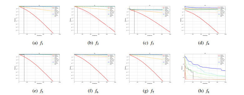
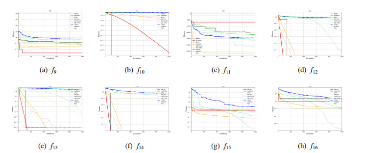
Aiming at the premature convergence problem of particle swarm optimization algorithm, a multi-sample particle swarm optimization (MSPSO) algorithm based on electric field force is proposed. Firstly, we introduce the concept of the electric field into the particle swarm optimization algorithm. The particles are affected by the electric field force, which makes the particles exhibit diverse behaviors. Secondly, MSPSO constructs multiple samples through two new strategies to guide particle learning. An electric field force-based comprehensive learning strategy (EFCLS) is proposed to build attractive samples and repulsive samples, thus improving search efficiency. To further enhance the convergence accuracy of the algorithm, a segment-based weighted learning strategy (SWLS) is employed to construct a global learning sample so that the particles learn more comprehensive information. In addition, the parameters of the model are adjusted adaptively to adapt to the population status in different periods. We have verified the effectiveness of these newly proposed strategies through experiments. Sixteen benchmark functions and eight well-known particle swarm optimization algorithm variants are employed to prove the superiority of MSPSO. The comparison results show that MSPSO has better performance in terms of accuracy, especially for high-dimensional spaces, while maintaining a faster convergence rate. Besides, a real-world problem also verified that MSPSO has practical application value.

| [1] |
O. Kaplan, E. Elik, Simplified model and genetic algorithm based simulated annealing approach for excitation current estimation of synchronous motor, Adv. Electr. Comput. Eng., 18 (2018), 75–84. doi: 10.4316/AECE.2018.04009

|
| [2] |
N. Mohamed, N. Bilel, A. S. Alsagri, A multi-objective methodology for multi-criteria engineering design, Appl. Soft Comput., 91 (2020), 106204. doi: 10.1016/j.asoc.2020.106204
|
| [3] |
E. Çelik, N. Öztürk, Y. Arya, Advancement of the search process of salp swarm algorithm for global optimization problems, Expert Syst. Appl., 182 (2021), 115292. doi: 10.1016/j.eswa.2021.115292
|
| [4] |
E. Çelik, Improved stochastic fractal search algorithm and modified cost function for automatic generation control of interconnected electric power systems, Eng. Appl. Artif. Intell., 88 (2020), 103407. doi: 10.1016/j.engappai.2019.103407
|
| [5] | G. Lin, J. Guan, An integrated method based on PSO and EDA for the max-cut problem, Comput. Intell. Neurosci., 2016 (2016), 3420671. |
| [6] |
E. Çelik, A powerful variant of symbiotic organisms search algorithm for global optimization, Eng. Appl. Artif. Intell., 87 (2020), 103294. doi: 10.1016/j.engappai.2019.103294
|
| [7] |
E. Çelik, N. Öztürk, A hybrid symbiotic organisms search and simulated annealing technique applied to efficient design of PID controller for automatic voltage regulator, Soft Comput., 22 (2018), 8011–8024. doi: 10.1007/s00500-018-3432-2
|
| [8] | N. Singh, S. B. Singh, E. H. Houssein, Hybridizing salp swarm algorithm with particle swarm optimization algorithm for recent optimization functions, Evol. Intell., (2020), 1–34. |
| [9] | J. Kennedy, R. Eberhart, Particle swarm optimization, in Proceedings of ICNN'95-international conference on neural networks, IEEE, (1995), 1942–1948. |
| [10] | P. Taylan, B. Akteke-Ozturk, Mathematical and data mining contributions to dynamics and optimization of gene-environment networks, Int. J. Theor. Phys., 4 (2007), 115–146. |
| [11] | E. Kropat, G. W. Weber, B. Akteke-Öztürk, Eco-finance networks under uncertainty, in Proceedings of the international conference on engineering optimization, (2008). |
| [12] |
G. W. Weber, İ. Batmaz, G. Köksal, P. Taylan, CMARS: A new contribution to nonparametric regression with multivariate adaptive regression splines supported by continuous optimization, Inverse Probl. Sci. Eng., 20 (2012), 371–400. doi: 10.1080/17415977.2011.624770
|
| [13] |
A. Özmen, G. W. Weber, İ. Batmaz, E. Kropat, RCMARS: Robustification of CMARS with different scenarios under polyhedral uncertainty set, Commun. Nonlinear Sci. Numer. Simul., 16 (2011), 4780–4787. doi: 10.1016/j.cnsns.2011.04.001
|
| [14] |
A. Özmen, E. Kropat, G. W. Weber, Robust optimization in spline regression models for multi-model regulatory networks under polyhedral uncertainty, Optimization, 66 (2017), 2135–2155. doi: 10.1080/02331934.2016.1209672
|
| [15] |
E. Kropat, G. W. Weber, E. B. Tirkolaee, Foundations of semialgebraic gene-environment networks, J. Dynam. Games, 7 (2020), 253. doi: 10.3934/jdg.2020018
|
| [16] |
R. K. Agrawal, B. Kaur, P. Agarwal, Quantum inspired Particle Swarm Optimization with guided exploration for function optimization, Appl. Soft Comput., 102 (2021), 107122. doi: 10.1016/j.asoc.2021.107122
|
| [17] |
Y. Du, F. Xu, A hybrid multi-step probability selection particle swarm optimization with dynamic chaotic inertial weight and acceleration coefficients for numerical function optimization, Symmetryn, 12 (2020), 922. doi: 10.3390/sym12060922
|
| [18] |
D. Tian, X. Zhao, Z. Shi, Chaotic particle swarm optimization with sigmoid-based acceleration coefficients for numerical function optimization, Swarm Evol. Comput., 51 (2019), 100573. doi: 10.1016/j.swevo.2019.100573
|
| [19] |
C. Wu, F. Yang, Y. Wu, R. Han, Prediction of crime tendency of high-risk personnel using C5. 0 decision tree empowered by particle swarm optimization, Math. Biosci. Eng., 16 (2019), 4135–4150. doi: 10.3934/mbe.2019206
|
| [20] |
M. Zhu, K. Wu, Y. Zhou, Z. Wang, J. Qiao, et al., Prediction of cooling moisture content after cut tobacco drying process based on a particle swarm optimization-extreme learning machine algorithm, Math. Biosci. Eng., 18 (2021), 2496–2507. doi: 10.3934/mbe.2021127
|
| [21] |
P. Singh, S. Chaudhury, B. K. Panigrahi, Hybrid MPSO-CNN: Multi-level Particle Swarm optimized Hyperparameters of Convolutional Neural Network, Swarm Evol. Comput., 63 (2021), 100863. doi: 10.1016/j.swevo.2021.100863
|
| [22] | J. Rojas-Delgado, R. Trujillo-Rasúa, Training Neural Networks by Continuation Particle Swarm Optimization, in International Workshop on Artificial Intelligence and Pattern Recognition, Springer, (2018), 59–67. |
| [23] |
T. L. Dang, Y. Hoshino, Hardware/software co-design for a neural network trained by particle swarm optimization algorithm, Neural Process Lett., 49 (2019), 481–505. doi: 10.1007/s11063-018-9826-4
|
| [24] |
L. M. Abualigah, A. T. Khader, E. S. Hanandeh, A new feature selection method to improve the document clustering using particle swarm optimization algorithm, J. Comput. Sci., 25 (2018), 456–466. doi: 10.1016/j.jocs.2017.07.018
|
| [25] |
M. A. Tawhid, K. B. Dsouza, Hybrid binary bat enhanced particle swarm optimization algorithm for solving feature selection problems, Appl. Comput. Inform., 16 (2018), 117–136. doi: 10.1016/j.aci.2018.04.001
|
| [26] |
F. Kılıç, Y. Kaya, S. Yildirim, A novel multi population based particle swarm optimization for feature selection, Knowl. Based Syst., 219 (2021), 106894. doi: 10.1016/j.knosys.2021.106894
|
| [27] |
X. Wang, Y. Li, Chaotic image encryption algorithm based on hybrid multi-objective particle swarm optimization and DNA sequence, Opt. Lasers Eng., 137 (2021), 106393. doi: 10.1016/j.optlaseng.2020.106393
|
| [28] |
H. T. Yau, T. H. Hung, C. C. Hsieh, Bluetooth based chaos synchronization using particle swarm optimization and its applications to image encryption, Sensors, 12 (2012), 7468–7484. doi: 10.3390/s120607468
|
| [29] | J. J. Liang, P. N. Suganthan, Dynamic multi-swarm particle swarm optimizer, in Proceedings 2005 IEEE Swarm Intelligence Symposium, IEEE, (2005), 124–129. |
| [30] |
S. Wang, G. Liu, M. Gao, S. Cao, A. Guo, J. Wang, Heterogeneous comprehensive learning and dynamic multi-swarm particle swarm optimizer with two mutation operators, Inf. Sci., 540 (2020), 175–201. doi: 10.1016/j.ins.2020.06.027
|
| [31] |
Q. Zhang, H. G. Li, An improved least squares SVM with adaptive PSO for the prediction of coal spontaneous combustion, Math. Biosci. Eng., 16 (2019), 3169–3182. doi: 10.3934/mbe.2019157
|
| [32] |
K. M. Ang, W. H. Lim, N. A. M. Isa, S. S. Tiang, C. H. Wong, A constrained multi-swarm particle swarm optimization without velocity for constrained optimization problems, Expert Syst. Appl., 140 (2020), 112882. doi: 10.1016/j.eswa.2019.112882
|
| [33] |
K. Chen, F. Zhou, A. Liu, Chaotic dynamic weight particle swarm optimization for numerical function optimization, Knowl. Based Syst., 139 (2018), 23–40. doi: 10.1016/j.knosys.2017.10.011
|
| [34] |
K. Zhang, Q. Huang, Y. Zhang, Enhancing comprehensive learning particle swarm optimization with local optima topology, Inf. Sci., 471 (2019), 1–18. doi: 10.1016/j.ins.2018.08.049
|
| [35] | S. Zhu, S. Zhou, J. Shang, L. Wang, B. Qiang, A multiion particle swarm optimization algorithm based on repellent and attraction forces, Concurr. Comput., 33 (2021), e5979. |
| [36] |
W. Li, X. Meng, Y. Huang, Z. H. Fu, Multipopulation cooperative particle swarm optimization with a mixed mutation strategy, Inf. Sci., 529 (2020), 179–196. doi: 10.1016/j.ins.2020.02.034
|
| [37] |
X. Xia, L. Gui, G. He, B. Wei, Y. Zhang, F. Yu, H. Wu, Z. H. Zhan, An expanded particle swarm optimization based on multi-exemplar and forgetting ability, Inf. Sci., 508 (2020), 105–120. doi: 10.1016/j.ins.2019.08.065
|
| [38] | Y. Shi, R. C. Eberhart, Parameter selection in particle swarm optimization, in International conference on evolutionary programming, Springer, (1998), 591–600. |
| [39] | M. U. Farooq, A. Ahmad, A. Hameed, Opposition-based initialization and a modified pattern for Inertia Weight (IW) in PSO, in 2017 IEEE International Conference on INnovations in Intelligent SysTems and Applications (INISTA), IEEE, (2017), 96–101. |
| [40] |
A. Chatterjee, P. Siarry, Nonlinear inertia weight variation for dynamic adaptation in particle swarm optimization, Comput. Oper. Res., 33 (2006), 859–871. doi: 10.1016/j.cor.2004.08.012
|
| [41] |
J. J. Liang, A. K. Qin, P. N. Suganthan, S. Baskar, Comprehensive learning particle swarm optimizer for global optimization of multimodal functions, IEEE Trans. Evol. Comput., 10 (2006), 281–295. doi: 10.1109/TEVC.2005.857610
|
| [42] | J. Zhou, W. Fang, X. Wu, J. Sun, S. Cheng, An opposition-based learning competitive particle swarm optimizer, in 2016 IEEE Congress on Evolutionary Computation (CEC), IEEE, (2016), 515–521. |
| [43] |
Q. Yang, W. N. Chen, T. Gu, H. Zhang, J. D. Deng, Y. Li, J. Zhang, Segment-Based Predominant Learning Swarm Optimizer for Large-Scale Optimization, IEEE Trans. Cybern., 47 (2017), 2896–2910. doi: 10.1109/TCYB.2016.2616170
|
| [44] | Y. Shi, R. Eberhart, A modified particle swarm optimizer, in IEEE world congress on computational intelligence, IEEE, (1998), 69–73. |
| [45] |
M. L. Dukic, Z. S. Dobrosavljevic, A method of a spread-spectrum radar polyphase code design, IEEE J. Sel. Areas Commun., 8 (1990), 743–749. doi: 10.1109/49.56381
|
| [46] |
S. Gil-López, J. Del Ser, S. Salcedo-Sanz, Á. M. Pérez-Bellido, J. Marı, J. A. Portilla-Figueras, et al., A hybrid harmony search algorithm for the spread spectrum radar polyphase codes design problem, Expert Syst. Appl., 39 (2012), 11089–11093. doi: 10.1016/j.eswa.2012.03.063
|
Figures(6) / Tables(10)

Shangbo Zhou, Yuxiao Han, Long Sha, Shufang Zhu. A multi-sample particle swarm optimization algorithm based on electric field force[J]. Mathematical Biosciences and Engineering, 2021, 18(6): 7464-7489. doi: 10.3934/mbe.2021369


 DownLoad: