AI-HydSu: An advanced hybrid approach using support vector regression and particle swarm optimization for dissolved oxygen forecasting

Dashe Li; Xueying Wang; Jiajun Sun; Huanhai Yang; Dashe Li; Xueying Wang; Jiajun Sun; Huanhai Yang

doi:10.3934/mbe.2021182

Mathematical Biosciences and Engineering

2021, Volume 18, Issue 4: 3646-3666. doi: 10.3934/mbe.2021182

Previous Article Next Article

Research article

AI-HydSu: An advanced hybrid approach using support vector regression and particle swarm optimization for dissolved oxygen forecasting

1.
School of Computer Science and Technology, Shandong Technology and Business University, Yantai 264005, China
2.
Co-innovation Center of Shandong Colleges and Universities: Future Intelligent Computing, Yantai 264005, China

Academic Editor: Yang Kuang

Received: 07 March 2021 Accepted: 19 April 2021 Published: 26 April 2021

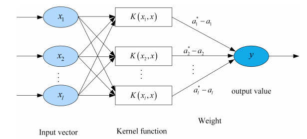
Since the variations in the dissolved oxygen concentration are affected by many factors, the corresponding uncertainty is nonlinear and fuzzy. Therefore, the accurate prediction of dissolved oxygen concentrations has been a difficult problem in the fishing industry. To address this problem, a hybrid dissolved oxygen concentration prediction model (AI-HydSu) is proposed in this paper. First, to ensure the accuracy of the experimental results, the data are preprocessed by wavelet threshold denoising, and the advantages of the particle swarm optimization (PSO) algorithm are used to search the solution space and select the best parameters for the support vector regression (SVR) model. Second, the prediction model optimizes the invariant learning factors in the standard PSO algorithm by using nonlinear adaptive learning factors, thus effectively preventing the algorithm from falling to local optimal solutions and accelerating the algorithm's optimization search process. Third, the velocities and positions of the particles are updated by constantly updating the learning factors to finally obtain the optimal combination of SVR parameters. The algorithm not only performs searches for the penalty factor, kernel function parameters, and error parameters in SVR but also balances its global and local search abilities. A dissolved oxygen concentration prediction experiment demonstrates that the proposed model achieves high accuracy and a fast convergence rate.
- support vector regression,
- particle swarm optimization,
- dissolved oxygen,
- adaptive,
- hybrid forecasting model
Citation: Dashe Li, Xueying Wang, Jiajun Sun, Huanhai Yang. AI-HydSu: An advanced hybrid approach using support vector regression and particle swarm optimization for dissolved oxygen forecasting[J]. Mathematical Biosciences and Engineering, 2021, 18(4): 3646-3666. doi: 10.3934/mbe.2021182

Related Papers:

Abstract

Since the variations in the dissolved oxygen concentration are affected by many factors, the corresponding uncertainty is nonlinear and fuzzy. Therefore, the accurate prediction of dissolved oxygen concentrations has been a difficult problem in the fishing industry. To address this problem, a hybrid dissolved oxygen concentration prediction model (AI-HydSu) is proposed in this paper. First, to ensure the accuracy of the experimental results, the data are preprocessed by wavelet threshold denoising, and the advantages of the particle swarm optimization (PSO) algorithm are used to search the solution space and select the best parameters for the support vector regression (SVR) model. Second, the prediction model optimizes the invariant learning factors in the standard PSO algorithm by using nonlinear adaptive learning factors, thus effectively preventing the algorithm from falling to local optimal solutions and accelerating the algorithm's optimization search process. Third, the velocities and positions of the particles are updated by constantly updating the learning factors to finally obtain the optimal combination of SVR parameters. The algorithm not only performs searches for the penalty factor, kernel function parameters, and error parameters in SVR but also balances its global and local search abilities. A dissolved oxygen concentration prediction experiment demonstrates that the proposed model achieves high accuracy and a fast convergence rate.

References

[1]	F. Khademi, M. Akbari, S. M. Jamal, M. Nikoo, Multiple linear regression, artificial neural network, and fuzzy logic prediction of 28 days compressive strength of concrete, Front. Struct. Civ. Eng., 11 (2017), 90–99. doi: 10.1007/s11709-016-0363-9
[2]	R. Pino-Mejías, A. Pérez-Fargallo, C. Rubio-Bellido, Jesús A. Pulido-Arcas, Comparison of linear regression and artificial neural networks models to predict heating and cooling energy demand, energy consumption and CO$_{2}$ emissions, Energy, 118 (2017), 24–36. doi: 10.1016/j.energy.2016.12.022
[3]	P. Singh, P. Gupta, K. Jyoti, TASM: technocrat ARIMA and SVR model for workload prediction of web applications in cloud, Cluster Comput., 22 (2019), 619–633. doi: 10.1007/s10586-018-2868-6
[4]	Y. Wang, C. H. Wang, C. Z. Shi, B. H. Xiao, Short-term cloud coverage prediction using the ARIMA time series model, Remote Sens. Lett., 9 (2018), 274–283. doi: 10.1080/2150704X.2017.1418992
[5]	L. Yang, H. Chen, Fault diagnosis of gearbox based on RBF-PF and particle swarm optimization wavelet neural network, Neural Comput. Appl., 31 (2019), 4463–4478. doi: 10.1007/s00521-018-3525-y
[6]	G. Renata, S. L. Zhu, S. Bellie, Forecasting river water temperature time series using a wavelet–neural network hybrid modelling approach, J. Hydrol., 578 (2019), 124115. doi: 10.1016/j.jhydrol.2019.124115
[7]	A. M. Zador, A critique of pure learning and what artificial neural networks can learn from animal brains, Nat. Commun., 10 (2019), 3770. doi: 10.1038/s41467-019-11786-6
[8]	A. Shebani, S. Iwnicki, Prediction of wheel and rail wear under different contact conditions using artificial neural networks, Wear, 406–407 (2018), 173–184.
[9]	E. Olyaie, H. Z. Abyaneh, A. D. Mehr, A comparative analysis among computational intelligence techniques for dissolved oxygen prediction in Delaware River, Geosci. Front., 8 (2017), 517–527. doi: 10.1016/j.gsf.2016.04.007
[10]	O. Kisi, M. Alizamir, A. D. Gorgij, Dissolved oxygen prediction using a new ensemble method, Environ. Sci. Pollut. Res. Int., 27 (2020), 9589–9603. doi: 10.1007/s11356-019-07574-w
[11]	B. Raheli, M. T. Aalami, A. El-Shafie, M. A. Ghorbani, R. C. Deo, Uncertainty assessment of the multilayer perceptron (MLP) neural network model with implementation of the novel hybrid MLP-FFA method for prediction of biochemical oxygen demand and dissolved oxygen: a case study of Langat River, Environ. Earth. Sci., 76 (2017), 503. doi: 10.1007/s12665-017-6842-z
[12]	A. A. Masrur Ahmed, Prediction of dissolved oxygen in Surma River by biochemical oxygen demand and chemical oxygen demand using the artificial neural networks (ANNs), J. King Saud Univ. Eng. Sci., 29 (2017), 151–158. doi: 10.1016/j.jksus.2016.05.002
[13]	B. Keshtegar, S. Heddam, Modeling daily dissolved oxygen concentration using modified response surface method and artificial neural network: a comparative study, Neural Comput. Appli., 30 (2018), 2995–3006. doi: 10.1007/s00521-017-2917-8
[14]	A. Csábrági, S. Molnár, P. Tanos, J. Kovács, Application of artificial neural networks to the forecasting of dissolved oxygen content in the Hungarian section of the river Danube, Ecol. Eng., 100 (2017), 63–72. doi: 10.1016/j.ecoleng.2016.12.027
[15]	S. Heddam, O. Kisi, Extreme learning machines: a new approach for modeling dissolved oxygen (DO) concentration with and without water quality variables as predictors, Environ. Sci. Pollut. Res., 24 (2017), 16702–16724. doi: 10.1007/s11356-017-9283-z
[16]	I. Ahmad, M. Basheri, M. J. Iqbal, A. Rahim, Performance comparison of support vector machine, random forest, and extreme learning machine for intrusion detection, IEEE Access, 6 (2018), 33789–33795. doi: 10.1109/ACCESS.2018.2841987
[17]	X. Luo, D. Li, S. Zhang, Traffic Flow Prediction during the Holidays Based on DFT and SVR, J. Sensors, 2019 (2019), 6461450.
[18]	M. S. Ahmad, S. M. Adnan, S. Zaidi, P. Bhargava, A novel support vector regression (SVR) model for the prediction of splice strength of the unconfined beam specimens, Constr. Build. Mater., 248 (2020), 118475. doi: 10.1016/j.conbuildmat.2020.118475
[19]	Y. Zhang, H. Sun, Y. Guo, Wind power prediction based on PSO-SVR and grey combination model, IEEE Access, 7 (2019), 136254–136267. doi: 10.1109/ACCESS.2019.2942012
[20]	E. Dodangeh, M. Panahi, F. Rezaie, S. Lee, D. T. Bui, C. W. Lee, et al., Novel hybrid intelligence models for flood-susceptibility prediction: Meta optimization of the GMDH and SVR models with the genetic algorithm and harmony search, J. Hydrol., 590 (2020), 125423. doi: 10.1016/j.jhydrol.2020.125423
[21]	Y. Xiang, L. Gou, L. He, S. Xia, W. Wang, A SVR–ANN combined model based on ensemble EMD for rainfall prediction, Appl. Soft Comput., 73 (2018), 874–883. doi: 10.1016/j.asoc.2018.09.018
[22]	M. Panahi, N. Sadhasivam, H. R. Pourghasemi, F. Rezaie, S. Lee, Spatial prediction of groundwater potential mapping based on convolutional neural network (CNN) and support vector regression (SVR), J. Hydrol., 588 (2020), 125033. doi: 10.1016/j.jhydrol.2020.125033
[23]	J. Kennedy, Particle swarm optimization, in Proceedings of ICNN'95 - International Conference on Neural Networks (R. Eberhart), (1995), 1942–1948.
[24]	X. Liang, T. Qi, Z. Jin, W. Qian, Hybrid support vector machine optimization model for inversion of tunnel transient electromagnetic method, Math. Biosci. Eng., 17 (2020), 3998. doi: 10.3934/mbe.2020221
[25]	M. Rosendo, A hybrid Particle Swarm Optimization algorithm for combinatorial optimization problems, in IEEE Congress on Evolutionary Computation (A. Pozo), (2010), 1–8.
[26]	C. F. Wang, K. Liu, A novel particle swarm optimization algorithm for global optimization, Comput. Intell. Neurosci., 2016 (2016), 9482073.
[27]	D. L. Donoho, I. M. Johnstone, Ideal spatial adaptation by wavelet shrinkage, Biometrika, 81 (1994), 425–455. doi: 10.1093/biomet/81.3.425
[28]	C. L. Wang, C. L. Zhang, P. T. Zhang, Denoising algorithm based on wavelet adaptive threshold, Phys. Procedia, 24 (2012), 678–685. doi: 10.1016/j.phpro.2012.02.100
[29]	S. Tomassini, A. Strazza, A. Sbrollini, I. Marcantoni, M. Morettini, S. Fioretti, et al., Wavelet filtering of fetal phonocardiography: A comparative analysis, Math. Biosci. Eng., 16 (2019), 6034. doi: 10.3934/mbe.2019302
[30]	F. M. Bayer, A. J. Kozakevicius, R. J. Cintra, An iterative wavelet threshold for signal denoising Signal Process., 162 (2019), 10–20.
[31]	H. Liu, L. Chang, C. Li, C. Yang, Particle swarm optimization-based support vector regression for tourist arrivals forecasting, Comput. Intell. Neurosci., 2018 (2018), 6076475.
[32]	A. T. C. Goh, Back-propagation neural networks for modeling complex systems, Artif. Intell. Eng., 9 (1995), 143–151. doi: 10.1016/0954-1810(94)00011-S
[33]	T. L. Lee, Back-propagation neural network for the prediction of the short-term storm surge in Taichung harbor, Taiwan, Eng. Appl. Artif. Intel., 21 (2008), 63–72. doi: 10.1016/j.engappai.2007.03.002
[34]	W. Hu, PSO-SVR: A Hybrid Short-term Traffic Flow Forecasting Method, in 2015 IEEE 21st International Conference on Parallel and Distributed Systems (ICPADS) (L. Yan), (2015), 553–561.
[35]	X. P. Hu, X. D. Dong, B. H. Yu, Method of optimal design with SVR-PSO for ultrasonic cutter assembly, Procedia CIRP, 50 (2016), 779–783. doi: 10.1016/j.procir.2016.04.180
[36]	K. Roosa, R. Luo, G. Chowell, Comparative assessment of parameter estimation methods in the presence of overdispersion: a simulation study, Math. Biosci. Eng., 16 (2019), 4229. doi: 10.3934/mbe.2019211
[37]	F. M. Butt, L. Hussain, A. Mahmood, K. J. Lone, Artificial Intelligence based accurately load forecasting system to forecast short and medium-term load demands, Math. Biosci. Eng., 18 (2021), 400. doi: 10.3934/mbe.2021022
[38]	H. Li, J. Tong, A novel clustering algorithm for time-series data based on precise correlation coefficient matching in the IoT, Math. Biosci. Eng., 16 (2019), 6654. doi: 10.3934/mbe.2019331
[39]	S. Zhu, M. Ptak, Z. M. Yaseen, J. Dai, B. Sivakumar, Forecasting surface water temperature in lakes: A comparison of approaches, J. Hydrol., 585 (2020), 124809. doi: 10.1016/j.jhydrol.2020.124809
[40]	J. Quilty, J. Adamowski, A stochastic wavelet-based data-driven framework for forecasting uncertain multiscale hydrological and water resources processes, Environ. Model Softw., 130 (2020), 104718. doi: 10.1016/j.envsoft.2020.104718
[41]	T. J. Glose, C. Lowry, M. B. Hausner, Examining the utility of continuously quantified Darcy fluxes through the use of periodic temperature time series, J. Hydrol., (2020), 125675.
[42]	F. Kang, J. Li, J. Dai, Prediction of long-term temperature effect in structural health monitoring of concrete dams using support vector machines with Jaya optimizer and salp swarm algorithms, Adv. Eng. Softw., 131 (2020), 60–67.
[43]	F. Kang, A. M. ASCE, J. Li, Displacement model for concrete dam safety monitoring via Gaussian process regression considering extreme air temperature, J. Struct. Eng., 146 (2020), 05019001. doi: 10.1061/(ASCE)ST.1943-541X.0002467

Reader Comments

Your name:*

Email:*
© 2021 the Author(s), licensee AIMS Press. This is an open access article distributed under the terms of the Creative Commons Attribution License (http://creativecommons.org/licenses/by/4.0)