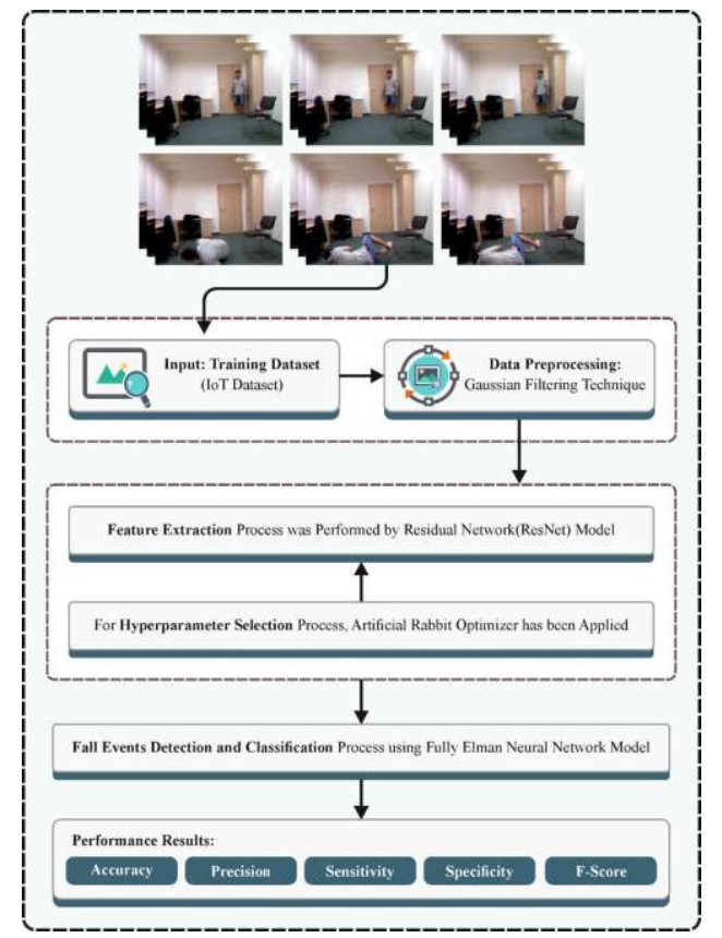
Fall detection (FD) for disabled persons in the Internet of Things (IoT) platform contains a combination of sensor technologies and data analytics for automatically identifying and responding to samples of falls. In this regard, IoT devices like wearable sensors or ambient sensors from the personal space role a vital play in always monitoring the user's movements. FD employs deep learning (DL) in an IoT platform using sensors, namely accelerometers or depth cameras, to capture data connected to human movements. DL approaches are frequently recurrent neural networks (RNNs) or convolutional neural networks (CNNs) that have been trained on various databases for recognizing patterns connected with falls. The trained methods are then executed on edge devices or cloud environments for real-time investigation of incoming sensor data. This method differentiates normal activities and potential falls, triggering alerts and reports to caregivers or emergency numbers once a fall is identified. We designed an Artificial Rabbit Optimizer with a DL-based FD and classification (ARODL-FDC) system from the IoT environment. The ARODL-FDC approach proposes to detect and categorize fall events to assist elderly people and disabled people. The ARODL-FDC technique comprises a four-stage process. Initially, the preprocessing of input data is performed by Gaussian filtering (GF). The ARODL-FDC technique applies the residual network (ResNet) model for feature extraction purposes. Besides, the ARO algorithm has been utilized for better hyperparameter choice of the ResNet algorithm. At the final stage, the full Elman Neural Network (FENN) model has been utilized for the classification and recognition of fall events. The experimental results of the ARODL-FDC technique can be tested on the fall dataset. The simulation results inferred that the ARODL-FDC technique reaches promising performance over compared models concerning various measures.
Citation: Eatedal Alabdulkreem, Mesfer Alduhayyem, Mohammed Abdullah Al-Hagery, Abdelwahed Motwakel, Manar Ahmed Hamza, Radwa Marzouk. Artificial Rabbit Optimizer with deep learning for fall detection of disabled people in the IoT Environment[J]. AIMS Mathematics, 2024, 9(6): 15486-15504. doi: 10.3934/math.2024749
Fall detection (FD) for disabled persons in the Internet of Things (IoT) platform contains a combination of sensor technologies and data analytics for automatically identifying and responding to samples of falls. In this regard, IoT devices like wearable sensors or ambient sensors from the personal space role a vital play in always monitoring the user's movements. FD employs deep learning (DL) in an IoT platform using sensors, namely accelerometers or depth cameras, to capture data connected to human movements. DL approaches are frequently recurrent neural networks (RNNs) or convolutional neural networks (CNNs) that have been trained on various databases for recognizing patterns connected with falls. The trained methods are then executed on edge devices or cloud environments for real-time investigation of incoming sensor data. This method differentiates normal activities and potential falls, triggering alerts and reports to caregivers or emergency numbers once a fall is identified. We designed an Artificial Rabbit Optimizer with a DL-based FD and classification (ARODL-FDC) system from the IoT environment. The ARODL-FDC approach proposes to detect and categorize fall events to assist elderly people and disabled people. The ARODL-FDC technique comprises a four-stage process. Initially, the preprocessing of input data is performed by Gaussian filtering (GF). The ARODL-FDC technique applies the residual network (ResNet) model for feature extraction purposes. Besides, the ARO algorithm has been utilized for better hyperparameter choice of the ResNet algorithm. At the final stage, the full Elman Neural Network (FENN) model has been utilized for the classification and recognition of fall events. The experimental results of the ARODL-FDC technique can be tested on the fall dataset. The simulation results inferred that the ARODL-FDC technique reaches promising performance over compared models concerning various measures.

| [1] | H. El Zein, F. Mourad-Chehade, H. Amoud, Leveraging Wi-Fi CSI Data for Fall Detection: A Deep Learning Approach, In 2023 5th International Conference on Bio-engineering for Smart Technologies (BioSMART), 2023, IEEE, 1–4. https://doi.org/10.1109/BioSMART58455.2023.10162090 |
| [2] |
J. Wang, W. C. Wang, K. W. Chau, L. Qiu, X. X. Hu, H. F. Zang, et al., An improved Golden Jackal Optimization Algorithm based on multi-strategy mixing for solving engineering optimization problems, J. Bionic Eng., 2024, 1–24. https://doi.org/10.1007/s42235-023-00469-0 doi: 10.1007/s42235-023-00469-0

|
| [3] | B. M. Sundaram, B. Rajalakshmi, R. K. Mandal, S. Nair, S. S. Choudhary, Fall Detection Among Elderly Using Deep Learning, In 2023 International Conference on Intelligent and Innovative Technologies in Computing, Electrical and Electronics (IITCEE), 554–558. IEEE, 2023. https://doi.org/10.1109/IITCEE57236.2023.10090887 |
| [4] |
Z. Lian, W. Wang, Z. Han, C. Su, Blockchain-based personalized federated learning for internet of medical things, IEEE T. Sust. Comput., 2023. https://doi.org/10.1109/TSUSC.2023.3279111 doi: 10.1109/TSUSC.2023.3279111
|
| [5] | F. Ahamed, S. Shahrestani, H. Cheung, Privacy-Aware IoT Based Fall Detection with Infrared Sensors and Deep Learning, In International Conference on Interactive Collaborative Robotics, Cham: Springer Nature Switzerland, 2023,392–401. https://doi.org/10.1007/978-3-031-35308-6_33 |
| [6] | W. C. Wang, L. Xu, K. W. Chau, Y. Zhao, D. M. Xu, An orthogonal opposition-based-learning Yin-Yang-pair optimization algorithm for engineering optimization, Eng. Comput., 2021, 1–35. |
| [7] | J. E. Rivadeneira, M. B. Jiménez, R. Marculescu, A. Rodrigues, F. Boavida, J. Sá Silva, A Blockchain-Based Privacy-Preserving Model for Consent and Transparency in Human-Centered Internet of Things, In Proceedings of the 8th ACM/IEEE Conference on Internet of Things Design and Implementation, 2023,301–314. https://doi.org/10.1145/3576842.3582379 |
| [8] |
M. Jarrah, H. Al Hamadi, A. Abu-Khadrah, T. M. Ghazal, IoMT-Based smart healthcare of elderly people using deep extreme learning machine, Comput. Mater. Con., 76 (2023). https://doi.org/10.32604/cmc.2023.032775 doi: 10.32604/cmc.2023.032775
|
| [9] |
W. Wang, W. Tian, K. W. Chau, Y. Xue, L. Xu, H. Zang, An improved bald eagle search algorithm with Cauchy mutation and adaptive weight factor for engineering optimization, Comput. Model. Eng. Sci., 136 (2023), 1603–1642. https://doi.org/10.32604/cmes.2023.026231 doi: 10.32604/cmes.2023.026231
|
| [10] |
B. Ozkaya, S. Duman, H. T. Kahraman, U. Guvenc, Optimal solution of the combined heat and power economic dispatch problem by adaptive fitness-distance balance based artificial rabbits optimization algorithm, Expert Syst. Appl., 238 (2024), 122272. https://doi.org/10.1016/j.eswa.2023.122272 doi: 10.1016/j.eswa.2023.122272
|
| [11] |
E. Alabdulkreem, R. Marzouk, M. Alduhayyem, M. A. Al-Hagery, A. Motwakel, M.A. Hamza, Chameleon Swarm Algorithm with improved fuzzy deep learning for fall detection approach to aid elderly people, J. Disabil. Res., 2 (2023), 62–70. https://doi.org/10.57197/JDR-2023-0020 doi: 10.57197/JDR-2023-0020
|
| [12] |
T. Vaiyapuri, E. L. Lydia, M. Y. Sikkandar, V. G. Díaz, I. V. Pustokhina, D. A. Pustokhin, Internet of things and deep learning enabled elderly fall detection model for smart homecare, IEEE Access, 9 (2021), 113879–113888. https://doi.org/10.1109/ACCESS.2021.3094243 doi: 10.1109/ACCESS.2021.3094243
|
| [13] |
R. Jain, V. B. Semwal, A novel feature extraction method for preimpact fall detection system using deep learning and wearable sensors, IEEE Sens. J., 22 (2022), 22943–22951. https://doi.org/10.1109/JSEN.2022.3213814 doi: 10.1109/JSEN.2022.3213814
|
| [14] |
F. Alotaibi, M. M. Alnfiai, F. N. Al-Wesabi, M. Alduhayyem, A. M. Hilal, M. A. Hamza, Internet of Things-driven Human Activity Recognition of elderly and disabled people using Arithmetic Optimization Algorithm with LSTM autoencoder, J. Disabil. Res., 2 (2023), 136–146. https://doi.org/10.1109/JSEN.2022.3213814 doi: 10.1109/JSEN.2022.3213814
|
| [15] | T. Xu, H. Se, J. Liu, A two-step fall detection algorithm combining threshold-based method and convolutional neural network, Metrol. Meas. Syst., 28 (2021). |
| [16] | A. R. Anwary, M. A. Rahman, A. J. M. Muzahid, A. W. U. Ashraf, M. Patwary, A. Hussain, Deep Learning enabled Fall Detection exploiting Gait Analysis, In 2022 44th Annual International Conference of the IEEE Engineering in Medicine & Biology Society (EMBC), IEEE, 2022, 4683–4686. https://doi.org/10.1109/EMBC48229.2022.9871964 |
| [17] |
T. Alanazi, G. Muhammad, Human fall detection using 3D multi-stream convolutional neural networks with fusion, Diagnostics, 12 (2022), 3060. https://doi.org/10.3390/diagnostics12123060 doi: 10.3390/diagnostics12123060
|
| [18] |
M. Al Duhayyim, Automated disabled people fall detection using Cuckoo Search with mobile networks, Intell. Autom. Soft Co., 36 (2023). https://doi.org/10.32604/iasc.2023.033585 doi: 10.32604/iasc.2023.033585
|
| [19] | H. Aboutalebi, H. Song, Y. Xie, A. Gupta, J. Sun, H. Su, et al., MAGID: An Automated Pipeline for Generating Synthetic Multi-modal Datasets, arXiv preprint arXiv: 2403.03194, 2024. |
| [20] |
R. Marzouk, F. Alrowais, F. N. Al-Wesabi, A. M. Hilal, Sign language recognition using Artificial Rabbits Optimizer with Siamese Neural Network for persons with disabilities, J. Disabil. Res., 2 (2023), 31–39. https://doi.org/10.57197/JDR-2023-0047 doi: 10.57197/JDR-2023-0047
|
| [21] |
V. Nyemeesha, B. M. Ismail, Implementation of noise and hair removals from dermoscopy images using hybrid Gaussian filter, Netw. Model. Anal. Health, 10 (2021), 1–10. https://doi.org/10.1007/s13721-021-00318-2 doi: 10.1007/s13721-021-00318-2
|
| [22] |
Y. Chen, Y. Lin, X. Xu, J. Ding, C. Li, Y. Zeng, et al., Classification of lungs infected COVID-19 images based on inception-ResNet, Comput. Meth. Prog. Bio., 225 (2022), 107053. https://doi.org/10.1016/j.cmpb.2022.107053 doi: 10.1016/j.cmpb.2022.107053
|
| [23] |
D. Izci, R. M. Rizk-Allah, V. Snášel, S. Ekinci, F. A. Hashim, L. Abualigah, A novel control scheme for automatic voltage regulator using novel modified Artificial Rabbits Optimizer, e-Prime-Advances in Electrical Engineering, Electron. Energy, 100325, 2023. https://doi.org/10.1016/j.cmpb.2022.107053 doi: 10.1016/j.cmpb.2022.107053
|
| [24] |
M. Fetanat, M. Stevens, P. Jain, C. Hayward, E. Meijering, N. H. Lovell, Fully Elman neural network: A novel deep recurrent neural network optimized by an improved Harris Hawks algorithm for classification of pulmonary arterial wedge pressure, IEEE T. Biomed. Eng., 69 (2021), 1733–1744. https://doi.org/10.1109/TBME.2021.3129459 doi: 10.1109/TBME.2021.3129459
|
| [25] | E. Auvinet, C. Rougier, J. Meunier, A. St-Arnaud, J. Rousseau, Multiple cameras fall dataset, Technical report 1350, DIRO - Université de Montréal, July 2010. |
| [26] | http://fenix.ur.edu.pl/~mkepski/ds/uf.html |


Figures(12) / Tables(6)

Eatedal Alabdulkreem, Mesfer Alduhayyem, Mohammed Abdullah Al-Hagery, Abdelwahed Motwakel, Manar Ahmed Hamza, Radwa Marzouk. Artificial Rabbit Optimizer with deep learning for fall detection of disabled people in the IoT Environment[J]. AIMS Mathematics, 2024, 9(6): 15486-15504. doi: 10.3934/math.2024749


 DownLoad: