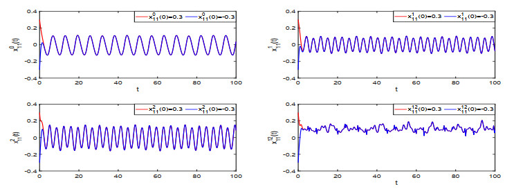
We adopted a non decomposition method to study the existence and stability of Stepanov almost periodic solutions in the distribution sense of stochastic shunting inhibitory cellular neural networks (SICNNs) with mixed time delays. Due to the lack of linear structure in the set composed of Stepanov almost periodic stochastic processes in the distribution sense. Due to the lack of linear structure in the set composed of distributed Stepanov periodic stochastic processes, it poses difficulties for the existence of Stepanov almost periodic solutions in the distribution sense of SICNNs. To overcome this difficulty, we first proved that the network under consideration has a unique solution in a space composed of $ \mathcal{L}^p $ bounded and $ \mathcal{L}^p $ uniformly continuous stochastic processes. Then, using stochastic analysis, inequality techniques, and the definition of Stepanov almost periodic stochastic processes in the distribution sense, we proved that this solution is also a Stepanov almost periodic solution in the distribution sense. Moreover, the result of the global exponential stability of this almost periodic solution is given. It is worth noting that even if the network under consideration degenerated into a real-valued network, our results are novel. Finally, we provided a numerical example to validate our theoretical findings.
Citation: Qi Shao, Yongkun Li. Almost periodic solutions for Clifford-valued stochastic shunting inhibitory cellular neural networks with mixed delays[J]. AIMS Mathematics, 2024, 9(5): 13439-13461. doi: 10.3934/math.2024655
We adopted a non decomposition method to study the existence and stability of Stepanov almost periodic solutions in the distribution sense of stochastic shunting inhibitory cellular neural networks (SICNNs) with mixed time delays. Due to the lack of linear structure in the set composed of Stepanov almost periodic stochastic processes in the distribution sense. Due to the lack of linear structure in the set composed of distributed Stepanov periodic stochastic processes, it poses difficulties for the existence of Stepanov almost periodic solutions in the distribution sense of SICNNs. To overcome this difficulty, we first proved that the network under consideration has a unique solution in a space composed of $ \mathcal{L}^p $ bounded and $ \mathcal{L}^p $ uniformly continuous stochastic processes. Then, using stochastic analysis, inequality techniques, and the definition of Stepanov almost periodic stochastic processes in the distribution sense, we proved that this solution is also a Stepanov almost periodic solution in the distribution sense. Moreover, the result of the global exponential stability of this almost periodic solution is given. It is worth noting that even if the network under consideration degenerated into a real-valued network, our results are novel. Finally, we provided a numerical example to validate our theoretical findings.

| [1] |
S. Blythe, X. R. Mao, X. X. Liao, Stability of stochastic delay neural networks, J. Franklin I., 338 (2001), 481–495. https://doi.org/10.1016/S0016-0032(01)00016-3 doi: 10.1016/S0016-0032(01)00016-3

|
| [2] |
X. X. Liao, X. Mao, Exponential stability and instability of stochastic neural networks, Stoch. Anal. Appl., 14 (1996), 165–185. https://doi.org/10.1080/07362999608809432 doi: 10.1080/07362999608809432
|
| [3] |
W. T. Wang, Further results on mean-square exponential Input-to-State stability of stochastic delayed Cohen-Grossberg neural networks, Neural Process. Lett., 55 (2023), 3953–3965. https://doi.org/10.1007/s11063-022-10974-8 doi: 10.1007/s11063-022-10974-8
|
| [4] |
T. Cai, P. Cheng, F. Q. Yao, M. G. Hua, Robust exponential stability of discrete-time uncertain impulsive stochastic neural networks with delayed impulses, Neural Netw., 160 (2023), 227–237. https://doi.org/10.1016/j.neunet.2023.01.016 doi: 10.1016/j.neunet.2023.01.016
|
| [5] |
F. H. Zhang, C. Fei, W. Y. Fei, Stability of stochastic Hopfield neural networks driven by G-Brownian motion with time-varying and distributed delays, Neurocomputing, 520 (2023), 320–330. https://doi.org/10.1016/j.neucom.2022.10.065 doi: 10.1016/j.neucom.2022.10.065
|
| [6] | A. Bouzerdoum, R. B. Pinter, Shunting inhibitory cellular neural networks: Derivation and stability analysis, IEEE Trans. Circuits Syst. I: Fundam. Theory Appl., 40 (1993), 215–221. |
| [7] |
C. X. Huang, S. G. Wen, L. H. Huang, Dynamics of anti-periodic solutions on shunting inhibitory cellular neural networks with multi-proportional delays, Neurocomputing, 357 (2019), 47–52. https://doi.org/10.1016/j.neucom.2019.05.022 doi: 10.1016/j.neucom.2019.05.022
|
| [8] |
Y. K. Li, X. F. Meng, Almost periodic solutions for quaternion-valued shunting inhibitory cellular neural networks of neutral type with time delays in the leakage term, Int. J. Syst. Sci., 49 (2018), 2490–2505. https://doi.org/10.1080/00207721.2018.1505006 doi: 10.1080/00207721.2018.1505006
|
| [9] | C. X. Huang, H. D. Yang, J. D. Cao, Weighted pseudo almost periodicity of multi-proportional delayed shunting inhibitory cellular neural networks with D operator, Discrete Contin. Dyn. Syst. S., 41 (2021), 1259–1272. |
| [10] |
X. Wang, X. Liang, X. Zhang, Y. Xue, Lp synchronization of shunting inhibitory cellular neural networks with multiple proportional delays, Inform. Sci., 654 (2024), 119865. https://doi.org/10.1016/j.ins.2023.119865 doi: 10.1016/j.ins.2023.119865
|
| [11] |
M. Akhmet, R. Seilova, M. Tleubergenova, A. Zhamanshin, Shunting inhibitory cellular neural networks with strongly unpredictable oscillations, Commun. Nonlinear Sci. Numer. Simulat., 89 (2020), 105287. https://doi.org/10.1016/j.cnsns.2020.105287 doi: 10.1016/j.cnsns.2020.105287
|
| [12] |
L. G. Yao, Global exponential convergence of neutral type shunting inhibitory cellular neural networks with D operator, Neural Process. Lett., 45 (2017), 401–409. https://doi.org/10.1007/s11063-016-9529-7 doi: 10.1007/s11063-016-9529-7
|
| [13] |
Y. K. Li, X. L. Huang, X. H. Wang, Weyl almost periodic solutions for quaternion-valued shunting inhibitory cellular neural networks with time-varying delays, AIMS Math., 7 (2022), 4861–4886. https://doi.org/10.3934/math.2022271 doi: 10.3934/math.2022271
|
| [14] |
X. H. Xu, Q. Xu, J. B. Yang, H. B. Xue, Y. H. Xu, Further research on exponential stability for quaternion-valued neural networks with mixed delays, Neurocomputing, 400 (2020), 186–205. https://doi.org/10.1016/j.neucom.2020.03.004 doi: 10.1016/j.neucom.2020.03.004
|
| [15] |
T. Peng, J. Q. Lu, Z. W. Tu, J. G. Lou, Finite-time stabilization of quaternion-valued neural networks with time delays: An implicit function method, Inform. Sci., 613 (2022), 747–762. https://doi.org/10.1016/j.ins.2022.09.014 doi: 10.1016/j.ins.2022.09.014
|
| [16] |
H. M. Wang, G. L. Wei, S. P. Wen, T. W. Huang, Impulsive disturbance on stability analysis of delayed quaternion-valued neural networks, Appl. Math. Comput., 390 (2021), 125680. https://doi.org/10.1016/j.amc.2020.125680 doi: 10.1016/j.amc.2020.125680
|
| [17] |
C. A. Popa, Global exponential stability of octonion-valued neural networks with leakage delay and mixed delays, Neural Netw., 105 (2018), 277–293. https://doi.org/10.1016/j.neunet.2018.05.006 doi: 10.1016/j.neunet.2018.05.006
|
| [18] |
S. S. Chouhan, R. Kumar, S. Sarkar, S. Das, Multistability analysis of octonion-valued neural networks with time-varying delays, Inform. Sci., 609 (2022), 1412–1434. https://doi.org/10.1016/j.ins.2022.07.123 doi: 10.1016/j.ins.2022.07.123
|
| [19] |
N. Huo, Y. K. Li, Finite-time Sp-almost periodic synchronization of fractional-order octonion-valued Hopfield neural networks, Chaos Soliton. Fract., 173 (2023), 113721. https://doi.org/10.1016/j.chaos.2023.113721 doi: 10.1016/j.chaos.2023.113721
|
| [20] |
B. Li, Y. W. Cao, Y. K. Li, Almost periodic oscillation in distribution for octonion-valued neutral-type stochastic recurrent neural networks with D operator, Nonlinear Dyn., 111 (2023), 11371–11388. https://doi.org/10.1007/s11071-023-08411-z doi: 10.1007/s11071-023-08411-z
|
| [21] | Y. K. Li, X. H. Wang, Besicovitch almost periodic stochastic processes and almost periodic solutions of Clifford-valued stochastic neural networks, Discrete Contin. Dyn. Syst. B, 28 (2023), 2154–2183. https://www.aimsciences.org/article/doi/10.3934/dcdsb.2022162 |
| [22] |
G. Rajchakit, R. Sriraman, C. P. Lim, B. Unyong, Existence, uniqueness and global stability of Clifford-valued neutral-type neural networks with time delays, Math. Comput. Simulat., 201 (2022), 508–527. https://doi.org/10.1016/j.matcom.2021.02.023 doi: 10.1016/j.matcom.2021.02.023
|
| [23] |
S. Y. Xing, H. Luan, F. Q. Deng, Global exponential stability for delayed Clifford-valued coupled neural networks with impulsive effects, J. Franklin I., 360 (2023), 14806–14822. https://doi.org/10.1016/j.jfranklin.2023.09.024 doi: 10.1016/j.jfranklin.2023.09.024
|
| [24] |
N. N. Zhao, Y. H. Qiao, Global exponential synchronization of Clifford-valued memristive fuzzy neural networks with delayed impulses, Cogn. Comput., 16 (2024), 671–681. https://doi.org/10.1007/s12559-023-10221-9 doi: 10.1007/s12559-023-10221-9
|
| [25] |
Y. Zhang, Y. H. Qiao, L. J. Duan, J. Miao, Multistability of almost periodic solution for Clifford-valued Cohen-Grossberg neural networks with mixed time delays, Chaos Soliton. Fract., 176 (2023), 114100. https://doi.org/10.1016/j.chaos.2023.114100 doi: 10.1016/j.chaos.2023.114100
|
| [26] |
S. Y. Xing, H. Luan, F. Q. Deng, Exponential synchronisation for delayed Clifford-valued coupled switched neural networks via static event-triggering rule, Int. J. Syst. Sci., 55 (2024), 1114–1126. https://doi.org/10.1080/00207721.2023.2301498 doi: 10.1080/00207721.2023.2301498
|
| [27] |
J. Li, H. Z. Zhao, Y. Zhang, S. T. Zhu, Y. Z. Zhang, Multistability of equilibrium points and periodic solutions for Clifford-valued memristive Cohen-Grossberg neural networks with mixed delays, Math. Method. Appl. Sci., 47 (2024), 2679–2701. https://doi.org/10.1002/mma.9772 doi: 10.1002/mma.9772
|
| [28] |
J. Gao, X. L. Huang, L. H. Dai, Weighted pseudo almost periodic synchronization for Clifford-valued neural networks with leakage delay and proportional delay, Acta Appl. Math., 186 (2023), 11. https://doi.org/10.1007/s10440-023-00587-1 doi: 10.1007/s10440-023-00587-1
|
| [29] |
B. Li, Y. N. Zhang, Y. K. Li, Besicovitch-like almost periodic solutions of Clifford-valued fuzzy cellular neural networks with time-varying delays, Franklin Open, 2 (2023), 100011. https://doi.org/10.1016/j.fraope.2023.100011 doi: 10.1016/j.fraope.2023.100011
|
| [30] |
H. L. Xu, B. Li, Pseudo almost periodic solutions for Clifford-valued neutral-type fuzzy neural networks with multi-proportional delay and D operator$^1$, J. Intell. Fuzzy Syst., 44 (2023), 2909–2925. https://doi.org/10.3233/JIFS-221017 doi: 10.3233/JIFS-221017
|
| [31] |
S. P. Shen, Y. K. Li, $S^{p}$-Almost periodic solutions of Clifford-valued fuzzy cellular neural networks with time-varying delays, Neural Process. Lett., 51 (2020), 1749–1769. https://doi.org/10.1007/s11063-019-10176-9 doi: 10.1007/s11063-019-10176-9
|
| [32] |
F. Chérif, M. Abdelaziz, Stepanov-like pseudo almost periodic solution of quaternion-valued for fuzzy recurrent neural networks with mixed delays, Neural Process. Lett., 51 (2020), 2211–2243. https://doi.org/10.1007/s11063-020-10193-z doi: 10.1007/s11063-020-10193-z
|
| [33] |
Y. K. Li, X. H. Wang, B. Li, Stepanov-like almost periodic dynamics of Clifford-valued stochastic fuzzy neural networks with time-varying delays, Neural Process. Lett., 54 (2022), 4521–4561. https://doi.org/10.1007/s11063-022-10820-x doi: 10.1007/s11063-022-10820-x
|
| [34] | A. Klenke, Probability theory: A comprehensive course, London: Springer Science & Business Media, 2008. |
| [35] | C. Corduneanu, Almost periodic oscillations and waves, New York: Springer Science & Business Media, 2009. |
| [36] | S. Hu, C. Huang, F. Wu, Stochastic differential equations, Beijing: Science Press, 2008. |
| [37] |
Y. K. Li, X. H. Wang, N. Huo, Weyl almost automorphic solutions in distribution sense of Clifford-valued stochastic neural networks with time-varying delays, P. Roy. Soc. A, 478 (2022), 20210719. https://doi.org/10.1098/rspa.2021.0719 doi: 10.1098/rspa.2021.0719
|


Figures(4)

Qi Shao, Yongkun Li. Almost periodic solutions for Clifford-valued stochastic shunting inhibitory cellular neural networks with mixed delays[J]. AIMS Mathematics, 2024, 9(5): 13439-13461. doi: 10.3934/math.2024655


 DownLoad: