Detecting isometries and symmetries of implicit algebraic surfaces

Uğur Gözütok; Hüsnü Anıl Çoban; Uğur Gözütok; Hüsnü Anıl Çoban

doi:10.3934/math.2024212

AIMS Mathematics

2024, Volume 9, Issue 2: 4294-4308. doi: 10.3934/math.2024212

Previous Article Next Article

Research article Special Issues

Detecting isometries and symmetries of implicit algebraic surfaces

Uğur Gözütok ^{1
,
,},
Hüsnü Anıl Çoban ²

1.
Department of Natural Sciences, National Defence University, İstanbul, Türkiye
2.
Department of Mathematics, Karadeniz Technical University, Trabzon, Türkiye

Received: 06 November 2023 Revised: 05 January 2024 Accepted: 09 January 2024 Published: 16 January 2024
MSC : 14Q10, 14Q20

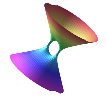
We presented a new and complete algorithm for detecting isometries and symmetries of implicit algebraic surfaces. First, our method reduced the problem to the case of isometries fixing the origin. Second, using tools from elimination theory and polynomial factoring, we determined the desired isometries between the surfaces. We have implemented the algorithm in Maple to provide evidences of the efficiency of the method.
- implicit surfaces,
- isometries,
- symmetries,
- equivalences,
- computer algebra
Citation: Uğur Gözütok, Hüsnü Anıl Çoban. Detecting isometries and symmetries of implicit algebraic surfaces[J]. AIMS Mathematics, 2024, 9(2): 4294-4308. doi: 10.3934/math.2024212

Related Papers:

Abstract

We presented a new and complete algorithm for detecting isometries and symmetries of implicit algebraic surfaces. First, our method reduced the problem to the case of isometries fixing the origin. Second, using tools from elimination theory and polynomial factoring, we determined the desired isometries between the surfaces. We have implemented the algorithm in Maple to provide evidences of the efficiency of the method.

References

[1]	J. G. Alcázar, C. Hermoso, G. Muntingh, Symmetry detection of rational space curves from their curvature and torsion, Comput. Aided Geom. D., 33 (2015), 51–65. https://doi.org/10.1016/j.cagd.2015.01.003 doi: 10.1016/j.cagd.2015.01.003
[2]	J. G. Alcázar, M. Lávi$\check{\text{c}}$ka, J. Vr$\check{\text{s}}$ek, Symmetries and similarities of planar algebraic curves using harmonic polynomials, J. Comput. Appl. Math., 357 (2019), 302–318. https://doi.org/10.1016/j.cam.2019.02.036 doi: 10.1016/j.cam.2019.02.036
[3]	J. G. Alcázar, E. Quintero, Affine equivalences of trigonometric curves, Acta Appl. Math., 170 (2020), 691–708. https://doi.org/10.1007/s10440-020-00354-6 doi: 10.1007/s10440-020-00354-6
[4]	J. G. Alcázar, E. Quintero, Affine equivalences, isometries and symmetries of ruled rational surfaces, J. Comput. Appl. Math., 364 (2020), 112339. https://doi.org/10.1016/j.cam.2019.07.004 doi: 10.1016/j.cam.2019.07.004
[5]	J. G. Alcázar, C. Hermoso, Computing projective equivalences of planar curves birationally equivalent to elliptic and hyperelliptic curves, Comput. Aided Geom. D., 91 (2021), 102048. https://doi.org/10.1016/j.cagd.2021.102048 doi: 10.1016/j.cagd.2021.102048
[6]	J. G. Alcázar, M. Lávi$\check{\text{c}}$ka, J. Vr$\check{\text{s}}$ek, Computing symmetries of implicit algebraic surfaces, Comput. Aided Geom. D., 104 (2023), 102221. https://doi.org/10.1016/j.cagd.2023.102221 doi: 10.1016/j.cagd.2023.102221
[7]	J. G. Alcázar, U. Gözütok, H. A. Çoban, C. Hermoso, Detecting affine equivalences between implicit planar algebraic curves, Acta Appl. Math., 182 (2022), 2. https://doi.org/10.1007/s10440-022-00539-1 doi: 10.1007/s10440-022-00539-1
[8]	J. G. Alcázar, C. Hermoso, Involutions of polynomially parametrized surfaces, J. Comput. Appl. Math., 294 (2016), 23–38. https://doi.org/10.1016/j.cam.2015.08.002 doi: 10.1016/j.cam.2015.08.002
[9]	M. Bizzarri, M. Làvi$\breve{\text{c}}$ka, J. Vr$\breve{\text{s}}$ek, Computing projective equivalences of special algebraic varieties, J. Comput. Appl. Math., 367 (2020), 112438. https://doi.org/10.1016/j.cam.2019.112438 doi: 10.1016/j.cam.2019.112438
[10]	M. Bizzarri, M. Làvi$\breve{\text{c}}$ka, J. Vr$\breve{\text{s}}$ek, Approximate symmetries of planar algebraic curves with inexact input, Comput. Aided Geom. D., 76 (2020), 101794. https://doi.org/10.1016/j.cagd.2019.101794 doi: 10.1016/j.cagd.2019.101794
[11]	M. Bizzarri, M. Làvi$\breve{\text{c}}$ka, J. Vr$\breve{\text{s}}$ek, Symmetries of discrete curves and point clouds via trigonometric interpolation, J. Comput. Appl. Math., 408 (2021), 114124. https://doi.org/10.1016/j.cam.2022.114124 doi: 10.1016/j.cam.2022.114124
[12]	M. Bizzarri, M. Làvi$\breve{\text{c}}$ka, J. Vr$\breve{\text{s}}$ek, Approximate symmetries of perturbed planar discrete curves, Comput. Aided Geom. D., 96 (2022), 102115. https://doi.org/10.1016/j.cagd.2022.102115 doi: 10.1016/j.cagd.2022.102115
[13]	H. S. M. Coxeter, Introduction to geometry, John Wiley & Sons, 1969.
[14]	D. Cox, J. Little, D. O'Shea, Ideals, varieties and algorithms, 2007.
[15]	U. Gözütok, H. A. Çoban, Y. Sa$\breve{\text{g}}$iro$\breve{\text{g}}$lu, J. G. Alcázar, A new method to detect projective equivalences and symmetries of rational $3D$ curves, J. Comput. Appl. Math., 419 (2023), 114782. https://doi.org/10.1016/j.cam.2022.114782 doi: 10.1016/j.cam.2022.114782
[16]	U$\breve{\text{g}}$ur Gözütok, https://www.ugurgozutok.com.
[17]	M. Hauer, B. Jüttler, Projective and affine symmetries and equivalences of rational curves in arbitrary dimension, J. Symb. Comput., 87 (2018), 68–86. https://doi.org/10.1016/j.jsc.2017.05.009 doi: 10.1016/j.jsc.2017.05.009
[18]	M. Hauer, B. Jüttler, J. Schicho, Projective and affine symmetries and equivalences of rational and polynomial surfaces, J. Comput. Appl. Math., 349 (2018), 424–437. https://doi.org/10.1016/j.cam.2018.06.026 doi: 10.1016/j.cam.2018.06.026
[19]	B. Jüttler, N. Lubbes, J. Schicho, Projective isomorphisms between rational surfaces, J. Algebra, 594 (2022), 571–596. https://doi.org/10.1016/j.jalgebra.2021.11.045 doi: 10.1016/j.jalgebra.2021.11.045
[20]	Maple^TM, 2021. Maplesoft, a division of Waterloo Maple Inc. Waterloo, Ontario.

Reader Comments

Your name:*

Email:*
© 2024 the Author(s), licensee AIMS Press. This is an open access article distributed under the terms of the Creative Commons Attribution License (http://creativecommons.org/licenses/by/4.0)