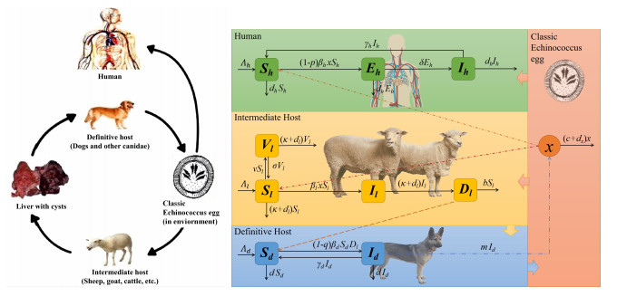
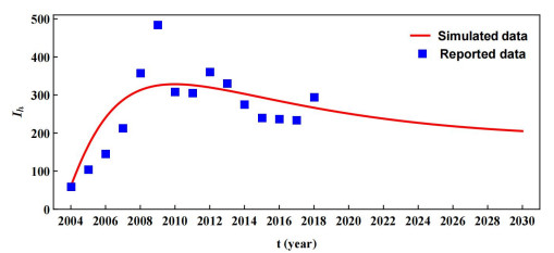
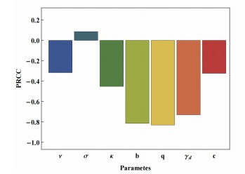
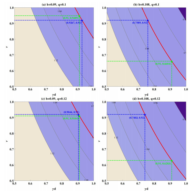
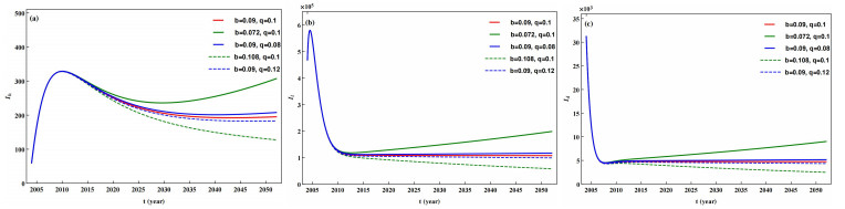
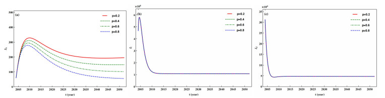
The prevention and control of the spread of Cystic Echinococcosis is an important public health issue. Health education has been supported by many governments because it can increase public awareness of echinococcosis, promote the development of personal hygiene habits, and subsequently reduce the transmission of echinococcosis. In this paper, a dynamic model of echinococcosis is used to integrate all aspects of health education. Theoretical analysis and numerical model fitting were used to quantitatively analysed by the impact of health education on the spread of echinococcosis. Theoretical findings indicate that the basic reproduction number is crucial in determining the prevalence of echinococcosis within a given geographical area. The parameters of the model were estimated and fitted by using data from the Ningxia Hui Autonomous Region in China, and the sensitivity of the basic reproduction number was analysed by using the partial rank correlation coefficient method. These findings illustrate that all aspects of health education demonstrate a negative correlation with the basic reproduction number, suggesting the effectiveness of health education in reducing the basic reproduction number and mitigating the transmission of echinococcosis, which is consistent with reality. Particularly, the basic reproduction number showed a strong negative correlation with the burial rate of infected livestock ($ b $) and the incidence of infected livestock viscera that is not fed to dogs ($ q $). This paper further analyzes the implementation plan for canine deworming rates and sheep immunity rates, as well as the transmission of infected hosts over time under different parameters $ b $ and $ q $. According to the findings, emphasizing the management of infected livestock in health education has the potential to significantly reduce the risk of echinococcosis transmission. This study will provide scientific support for the creation of higher quality health education initiatives.
Citation: Qianqian Cui, Qiang Zhang, Zengyun Hu. Modeling and analysis of Cystic Echinococcosis epidemic model with health education[J]. AIMS Mathematics, 2024, 9(2): 3592-3612. doi: 10.3934/math.2024176
The prevention and control of the spread of Cystic Echinococcosis is an important public health issue. Health education has been supported by many governments because it can increase public awareness of echinococcosis, promote the development of personal hygiene habits, and subsequently reduce the transmission of echinococcosis. In this paper, a dynamic model of echinococcosis is used to integrate all aspects of health education. Theoretical analysis and numerical model fitting were used to quantitatively analysed by the impact of health education on the spread of echinococcosis. Theoretical findings indicate that the basic reproduction number is crucial in determining the prevalence of echinococcosis within a given geographical area. The parameters of the model were estimated and fitted by using data from the Ningxia Hui Autonomous Region in China, and the sensitivity of the basic reproduction number was analysed by using the partial rank correlation coefficient method. These findings illustrate that all aspects of health education demonstrate a negative correlation with the basic reproduction number, suggesting the effectiveness of health education in reducing the basic reproduction number and mitigating the transmission of echinococcosis, which is consistent with reality. Particularly, the basic reproduction number showed a strong negative correlation with the burial rate of infected livestock ($ b $) and the incidence of infected livestock viscera that is not fed to dogs ($ q $). This paper further analyzes the implementation plan for canine deworming rates and sheep immunity rates, as well as the transmission of infected hosts over time under different parameters $ b $ and $ q $. According to the findings, emphasizing the management of infected livestock in health education has the potential to significantly reduce the risk of echinococcosis transmission. This study will provide scientific support for the creation of higher quality health education initiatives.

| [1] |
C. Liu, Y. Xu, A. M. Cadavid-Restrepo, Z. Lou, H. Yan, L. Li, et al., Estimating the prevalence of Echinococcus in domestic dogs in highly endemic for echinococcosis, Infect. Dis. Poverty., 7 (2018), 77. https://doi.org/10.1186/s40249-018-0458-8 doi: 10.1186/s40249-018-0458-8

|
| [2] |
X. Han, Q. Cai, W. Wang, H. Wang, Q. Zhang, Y. Wang, Childhood suffering: hyper endemic echinococcosis in Qinghai-Tibetan primary school students, China, Infect. Dis. Poverty., 7 (2018), 1. https://doi.org/10.1186/s40249-018-0455-y doi: 10.1186/s40249-018-0455-y
|
| [3] |
L. Xu, Y. Chen, F. Sun, A national survey on current status of the important parasitic diseases in human population, Chin, J. Parasitol. Parasit. Dis., 23 (2005), 332–340. https://doi.org/10.3969/j.issn.1000-7423.2005.z1.004 doi: 10.3969/j.issn.1000-7423.2005.z1.004
|
| [4] |
S. Han, Y. Kui, C. Xue, Y. Zhang, B. Zhang, Q. Li, et al., The endemic status of echinococcosis in China from 2004 to 2020, Chin J Parasitol Parasit Dis., 40 (2022), 475–480. https://doi.org/10.12140/j.issn.1000-7423.2022.04.009 doi: 10.12140/j.issn.1000-7423.2022.04.009
|
| [5] |
Q. Yu, N. Xiao, S. Han, T. Tian, X. Zhou, Progress on the national echinococcosis control programme in China: analysis of humans and dogs population intervention during 2004-2014, Infect. Dis. Poverty., 9 (2020), 137. https://doi.org/10.1186/s40249-020-00747-7 doi: 10.1186/s40249-020-00747-7
|
| [6] |
L. Wang, Report on the final evaluation of the 12th five-years action plan on echinococcosis and the 13th five-years control plan on echinococcosis, China Anim. Health Insp., 19 (2017), 13–19. https://doi.org/10.3969/j.issn.1008-4754.2017.07.004 doi: 10.3969/j.issn.1008-4754.2017.07.004
|
| [7] | T. C. Beard, The elimination of Echinococcosis from Iceland, Bull World Health Organ, 48 (1973), 653. |
| [8] |
P. S. Craig, D. Hegglin, M. W. Lightowlers, P. R. Torgerson, Q. Wang, Echinococcosis: control and prevention, Adv Parasit., 96 (2017), 55–158. https://doi.org/10.1016/bs.apar.2016.09.002 doi: 10.1016/bs.apar.2016.09.002
|
| [9] |
M. Qian, C. Zhou, H. Zhu, T. Zhu, J. Huang, Y. Chen, et al., Assessment of health education products aimed at controlling and preventing helminthiases in China, Infect. Dis. Poverty., 8 (2019), 22. https://doi.org/10.1186/s40249-019-0531-y doi: 10.1186/s40249-019-0531-y
|
| [10] |
Z. Jiumai, J. Li, H. Wu, H. Zeng, Q. Xu, P. Liu, et al., Effect evaluation of publicity film Gaisang M$\hat{\text{e}}$dog in buds on human echinococcosis prevention in pilot regions, China Anim. Health Insp., 34 (2017), 28–31. https://doi.org/10.3969/j.issn.1005-944X.2017.07.008 doi: 10.3969/j.issn.1005-944X.2017.07.008
|
| [11] |
P. Liu, Y. Wang, J. Kang, X. Huang, W. Ge, C. Li, et al., Evaluation on popularization effect of echinococcosis promotional film Galsang Flowers in Blossom, China Anim. Health Insp., 3 (2021), 1–4. https://doi.org/10.3969/j.issn.1005-944X.2021.07.001 doi: 10.3969/j.issn.1005-944X.2021.07.001
|
| [12] |
Q. Cui, Z. Shi, D. Yimamaidi, B. Hu, Z. Zhang, M. Saqib, et al., Dynamic variations in COVID-19 with the SARS-CoV-2 Omicron variant in Kazakhstan and Pakistan, Infect. Dis. Poverty., 12 (2023), 18. https://doi.org/10.1186/s40249-023-01072-5 doi: 10.1186/s40249-023-01072-5
|
| [13] |
R. Musa, O. J. Peter, F. A. Oguntolu, A non-linear differential equation model of COVID-19 and seasonal influenza co-infection dynamics under vaccination strategy and immunity waning, Healthcare Analytics, 4 (2023), 100240. https://doi.org/10.1016/j.health.2023.100240 doi: 10.1016/j.health.2023.100240
|
| [14] |
B. I. Omede, O. J. Peter, W. Atokolo, B. Bolaji, T. A. Ayoola, A mathematical analysis of the two-strain tuberculosis model dynamics with exogenous re-infection, Healthcare Analytics, 4 (2023), 100266. https://doi.org/10.1016/j.health.2023.100266 doi: 10.1016/j.health.2023.100266
|
| [15] |
K. Oshinubi, O. J. Peter, E. Addai, E. Mwizerwa, O. Babasola, I. V. Nwabufo, et al., Mathematical modelling of tuberculosis outbreak in an East African country incorporating vaccination and treatment, Computation, 11 (2023), 143. https://doi.org/10.3390/computation11070143 doi: 10.3390/computation11070143
|
| [16] |
O. J. Peter, H. S. Panigoro, A. Abidemi, Ma. M. Ojo, F. A. Oguntolu, Mathematical model of COVID-19 pandemic with double dose vaccination, Acta Biotheor., 71 (2023), 9. https://doi.org/10.1007/s10441-023-09460-y doi: 10.1007/s10441-023-09460-y
|
| [17] |
M. A. Gemmell, J. R. Lawson, M. G. Roberts, Population dynamics in Echinococcosis and cysticercosis: Biological parameters of Echinococcus granulosus in dogs and sheep, Parasitology, 92 (1986), 599–620. https://doi.org/10.1017/S0031182000065483 doi: 10.1017/S0031182000065483
|
| [18] |
M. A. Gemmell, J. R. Lawson, M. G. Roberts, B. R. Kerin, C. J. Mason, Population dynamics in Echinococcosis and cysticercosis: comparison of the response of Echinococcus granulosus, Taenia hydatigena and T.ovis to control, Parasitology, 93 (1986), 357–369. https://doi.org/10.1017/S0031182000051520 doi: 10.1017/S0031182000051520
|
| [19] |
M. A. Gemmell, J. R. Lawson, M. G. Roberts, Population dynamics in Echinococcosis and cysticercosis: Evaluation of the biological parameters of Taenia hydatigena and T. ovis and comparison with those of Echinococcus granulosus, Parasitology, 94 (1987), 161–180. https://doi.org/10.1017/S0031182000053543 doi: 10.1017/S0031182000053543
|
| [20] |
M. G. Roberts, J. R. Lawson, M. A. Gemmell, Population dynamics in echinococcosis and cysticercosis: mathematical model of the life-cycle of Echinococcus granulosus, Paraisitology, 92 (1986), 621–641. https://doi.org/10.1017/S0031182000065495 doi: 10.1017/S0031182000065495
|
| [21] |
M. G. Roberts, J. R. Lawson, M. A. Gemmell, opulation dynamics in echinococcosis and cysticercosis: Mathematical model of the life-cycles of Taenia hydatigena and T.ovis, Parasitology, 94 (1987), 181–197. https://doi.org/10.1017/S0031182000053555 doi: 10.1017/S0031182000053555
|
| [22] |
K. Wang, Z. Teng, X. Zhang, Dynamical behaviors of an Echinococcosis epidemic model with distributed delays, Math. Biosci. Eng., 14 (2017), 1425–1445. https://doi.org/10.3934/mbe.2017074 doi: 10.3934/mbe.2017074
|
| [23] |
K. Wang, X. Zhang, Z. Teng, L. Wang, L. Zhang, Analysis of a patch model for the dynamical transmission of echinococcosis, Abstr. Appl. Anal., 2014 (2014), 1–13. https://doi.org/10.1155/2014/576365 doi: 10.1155/2014/576365
|
| [24] |
J. Zhao, R. Yang, A dynamical model of echinococcosis with optimal control and cost-effectiveness, Nonlinear Anal.: Real., 62 (2021), 103388. https://doi.org/10.1016/j.nonrwa.2021.103388 doi: 10.1016/j.nonrwa.2021.103388
|
| [25] |
G. Zhu, S. Chen, B. Shi, H. Qiu, S. Xia, Dynamics of echinococcosis transmission among multiple species and a case study in Xinjiang, China, Chaos Soliton. Fract., 127 (2019), 103–109. https://doi.org/10.1016/j.chaos.2019.06.032 doi: 10.1016/j.chaos.2019.06.032
|
| [26] |
A. S. Hassan, J. M. W. Munganga, Mathematical global dynamics and control strategies on echinococcus multilocularis infection, Comput. Math. Methods Med., 2019 (2019), 3569528. https://doi.org/10.1155/2019/3569528 doi: 10.1155/2019/3569528
|
| [27] |
K. Wang, X. Zhang, Z. Jin, H. Ma, T. Teng, L. Wang, odeling and analysis of the transmission of Echinococcosis with application to Xinjiang Uygur Autonomous Region of China, J. Theor. Biol., 333 (2013), 78–90. https://doi.org/10.1016/j.jtbi.2013.04.020 doi: 10.1016/j.jtbi.2013.04.020
|
| [28] |
Y. He, Q. Cui, Z. Hu, Modeling and analysis of the transmission dynamics of cystic echinococcosis: Effects of increasing the number of sheep, Math. Biosci. Eng., 20 (2023), 14596–14615. https://doi.org/10.3934/mbe.2023653 doi: 10.3934/mbe.2023653
|
| [29] |
J. Sun, H. Zhang, D. Jiang, On the Dynamics Behaviors of a Stochastic Echinococcosis Infection Model with Environmental Noise, Discrete. Dyn. Nat. Soc., 2021 (2021), 1–18. https://doi.org/10.1155/2021/8204043 doi: 10.1155/2021/8204043
|
| [30] |
X. Rong, M. Fan, X. Sun, Y. Wang, H. Zhu, Impact of disposing stray dogs on risk assessment and control of Echinococcosis in Inner Mongolia, Math. Biosci., 299 (2018), 85–96. https://doi.org/10.1016/j.mbs.2018.03.008 doi: 10.1016/j.mbs.2018.03.008
|
| [31] |
X. Rong, M. Fan, H. Zhu, Y. Zheng, Dynamic modeling and optimal control of cystic echinocococcosis, Infect. Dis. Poverty., 10 (2021), 38. https://doi.org/10.1186/s40249-021-00807-6 doi: 10.1186/s40249-021-00807-6
|
| [32] |
Y. Zhang, Y. Xiao, Modeling and analyzing the effects of fixed-time intervention on transmission dynamics of echinococcosis in Qinghai province, Math. Method. Appl. Sci., 44 (2021), 4276–4296. https://doi.org/10.1002/mma.7029 doi: 10.1002/mma.7029
|
| [33] |
F. Porcu, C. Cantacessi, G. Dess, M. F. Sini, F. Ahmed, L. Cavallo, et al., 'Fight the parasite': Raising awareness of cystic echinococcosis in primary school children in endemic countries, Parasite. Vector., 15 (2022), 449. https://doi.org/10.1186/s13071-022-05575-2 doi: 10.1186/s13071-022-05575-2
|
| [34] |
J. E. Moss, X. Chen, T. Li, J. Qiu, Q. Wang, P. Giraudoux, Reinfection studies of canine echinococcosis and role of dogs in transmission of Echinococcus multilocularis in Tibetan communities, Sichuan, China, Parasitology, 140 (2013), 1685–1692. https://doi.org/10.1017/S0031182013001200 doi: 10.1017/S0031182013001200
|
| [35] |
O. Diekmann, J. A. P. Heesterbeek, J. A. Metz, On the definition and the computation of the basic reproduction ratio $R_0$ in the models for infectious disease inheterogeneous populations, J. Math. Biol., 28 (1990), 365–382. https://doi.org/10.1007/BF00178324 doi: 10.1007/BF00178324
|
| [36] |
V. D. P. Driessche, J. Watmough, Reproduction numbers and sub-threshold endemic equilibria for compartmental models of disease transmission, Math. Biosci., 180 (2002), 29–48. https://doi.org/10.1016/S0025-5564(02)00108-6 doi: 10.1016/S0025-5564(02)00108-6
|
| [37] |
H. R. Thieme, Convergence results and a Poincare-Bendixson trichotomy for asymptotically autonomous differential equations, J. Math. Biol., 30 (1992), 755–763. https://doi.org/10.1007/BF00173267 doi: 10.1007/BF00173267
|
| [38] | S. Wang, S. Ye, Text Book of Medical Microbiology and Parasitology, 1 Ed., Beijing: Science Press, 2006. http://refhub.elsevier.com/S0025-5564(17)30436-4/sbref0010 |
| [39] |
P. R. Torgerson, K. K. Burtisurnov, B. S. Shaikenov, A. T. Rysmukhambetova, A. M. Abdybekova, A. E. Ussenbayev, Modelling the transmission dynamics of echinococcus granulosus in sheep and cattle in Kazakhstan, Vet. Parasitol., 114 (2003), 143–153. https://doi.org/10.1016/S0304-4017(03)00136-5 doi: 10.1016/S0304-4017(03)00136-5
|
| [40] |
C. M. Budke, J. M. Qiu, Q. Wang, P. P. Torgerson, Economic effects of Echinococcosis in a disease-endemic region of the Tibetan Plateau, Am. J. Trop. Med. Hyg., 73 (2005), 2–10. https://doi.org/10.4269/ajtmh.2005.73.2 doi: 10.4269/ajtmh.2005.73.2
|
| [41] |
P. R. Torgerson, D. D. Heath, Transmission dynamics and control options for echinococcus granulosus, Parasitology, 127 (2013), 143–158. https://doi.org/10.1017/S0031182003003810 doi: 10.1017/S0031182003003810
|
| [42] |
W. Zhang, Z. Zhang, W. Wu, B. Shi, J. Li, X. Zhou, et al., Epidemiology and control of echinococcosis in Central Asia, with particular reference to the People's Republic of China, Acta Trop., 141 (2015), 235–243. https://doi.org/10.1016/j.actatropica.2014.03.014 doi: 10.1016/j.actatropica.2014.03.014
|
| [43] |
O. J. Peter, C. E. Madubueze, M. M. Ojo, F. A. Oguntolu, T. A. Ayoola, Modeling and optimal control of monkeypox with cost-effective strategies, Model. Earth. Syst. Env., 9 (2023), 1989–2007. https://doi.org/10.1007/s40808-022-01607-z doi: 10.1007/s40808-022-01607-z
|
Figures(6) / Tables(1)

Qianqian Cui, Qiang Zhang, Zengyun Hu. Modeling and analysis of Cystic Echinococcosis epidemic model with health education[J]. AIMS Mathematics, 2024, 9(2): 3592-3612. doi: 10.3934/math.2024176


 DownLoad: