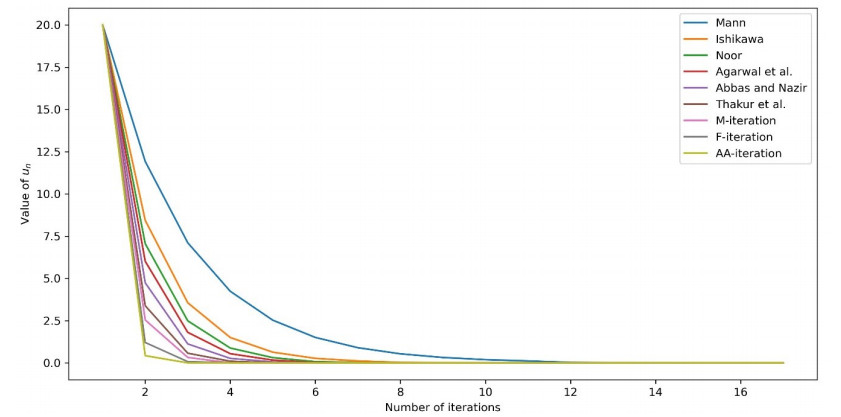
Loading [MathJax]/jax/output/SVG/jax.js
Research article Special Issues

The AA-iterative algorithm in hyperbolic spaces with applications to integral equations on time scales

  • We explored the AA-iterative algorithm within the hyperbolic spaces (HSs), aiming to unveil a stability outcome for contraction maps and convergence outcomes for generalized (α,β)-nonexpansive (GαβN) maps in such spaces. Through this algorithm, we derived compelling outcomes for both strong and Δ-convergence and weak w2-stability. Furthermore, we provided an illustrative example of GαβN maps and conducted a comparative analysis of convergence rates against alternative iterative methods. Additionally, we demonstrated the practical relevance of our findings by applying them to solve the linear Fredholm integral equations (FIEs) and nonlinear Fredholm-Hammerstein integral equations (FHIEs) on time scales.

    Citation: Aynur Şahin, Zeynep Kalkan. The AA-iterative algorithm in hyperbolic spaces with applications to integral equations on time scales[J]. AIMS Mathematics, 2024, 9(9): 24480-24506. doi: 10.3934/math.20241192

    Related Papers:

    [1] Nabil Kerdid . Asymptotic analysis of stretching modes for a folded plate. AIMS Mathematics, 2023, 8(10): 23974-23988. doi: 10.3934/math.20231222
    [2] Javier de Lucas, Julia Lange, Xavier Rivas . A symplectic approach to Schrödinger equations in the infinite-dimensional unbounded setting. AIMS Mathematics, 2024, 9(10): 27998-28043. doi: 10.3934/math.20241359
    [3] Muhammad Afzal, Tariq Ismaeel, Azhar Iqbal Kashif Butt, Zahid Farooq, Riaz Ahmad, Ilyas Khan . On the reducibility of a class of almost-periodic linear Hamiltonian systems and its application in Schrödinger equation. AIMS Mathematics, 2023, 8(3): 7471-7489. doi: 10.3934/math.2023375
    [4] Maxime Krier, Julia Orlik . Solvability of a fluid-structure interaction problem with semigroup theory. AIMS Mathematics, 2023, 8(12): 29490-29516. doi: 10.3934/math.20231510
    [5] Maha M. Helmi, Ali M. Mubaraki, Rahmatullah Ibrahim Nuruddeen . Analysis of horizontally polarized shear waves on a highly inhomogeneous loaded bi-material plate. AIMS Mathematics, 2023, 8(1): 2117-2136. doi: 10.3934/math.2023109
    [6] Nabil Kerdid . Asymptotic analysis of high frequency modes for thin elastic plates. AIMS Mathematics, 2023, 8(8): 18618-18630. doi: 10.3934/math.2023948
    [7] Min Zhang, Yi Wang, Yan Li . Reducibility and quasi-periodic solutions for a two dimensional beam equation with quasi-periodic in time potential. AIMS Mathematics, 2021, 6(1): 643-674. doi: 10.3934/math.2021039
    [8] Jia Li, Xia Li, Chunpeng Zhu . Reducibility for a class of almost periodic Hamiltonian systems which are degenerate. AIMS Mathematics, 2023, 8(1): 2296-2307. doi: 10.3934/math.2023119
    [9] Syed T. R. Rizvi, Sana Ghafoor, Aly R. Seadawy, Ahmed H. Arnous, Hakim AL Garalleh, Nehad Ali Shah . Exploration of solitons and analytical solutions by sub-ODE and variational integrators to Klein-Gordon model. AIMS Mathematics, 2024, 9(8): 21144-21176. doi: 10.3934/math.20241027
    [10] Aziz Ur Rehman, Muhammad Bilal Riaz, Ilyas Khan, Abdullah Mohamed . Time fractional analysis of Casson fluid with application of novel hybrid fractional derivative operator. AIMS Mathematics, 2023, 8(4): 8185-8209. doi: 10.3934/math.2023414
  • We explored the AA-iterative algorithm within the hyperbolic spaces (HSs), aiming to unveil a stability outcome for contraction maps and convergence outcomes for generalized (α,β)-nonexpansive (GαβN) maps in such spaces. Through this algorithm, we derived compelling outcomes for both strong and Δ-convergence and weak w2-stability. Furthermore, we provided an illustrative example of GαβN maps and conducted a comparative analysis of convergence rates against alternative iterative methods. Additionally, we demonstrated the practical relevance of our findings by applying them to solve the linear Fredholm integral equations (FIEs) and nonlinear Fredholm-Hammerstein integral equations (FHIEs) on time scales.


    The moderately thick plate is an important material that can adapt to high pressure, high temperature and strong radiation environments, often used in construction engineering, machinery manufacturing, container manufacturing and so on [1,2]. In recent years, many achievements have been made in numerical methods of moderately thick plate problems. There are some typical numerical methods, such as the meshless local radial point interpolation method [3], discrete singular convolution methods [4], spectral element method [5], meshless local Petrov-Galerkin method [6], differential quadrature element method [7], finite integral transform method [8] and chaotic radial basis function method [9]. Compared with numerical methods, the analytical method seems more accurate, but it is difficult to construct. Through the efforts of many scholars, the analytical method has made great progress. The common analytical methods are integral transformation [10,11], semi-inverse method [12], infinite series method [13] and Green's functions [14]. Traditionally, some analytical solutions always need to eliminate the unknown functions by various methods in the range of a class of variables so as to obtain a partial differential equation with higher order, which will make separating variables and other mathematical methods impossible. In order to avoid this phenomenon, academician Zhong put forward the SEA in the 1990s. The essence of SEA is the method of separation of variables based on Hamiltonian system, which does not need to assume the form of the solution in advance. The main feature of the approach is that the solution procedure is conducted in the symplectic space with dual variables rather than in the Euclidean space with one kind of variables, which is rational to solve the equations of elasticity [15,16]. Within the framework of the Hamiltonian system, the analytical solutions of the considered problem can be obtained by using the complete expansion of symplectic eigenvectors without any prior assumptions of the solution forms, which shows the distinctive advantage of the SEA.

    SEA needs to transform the equations of elasticity into a proper Hamiltonian system and can uniformly solve the state vector, including as many unknown functions, such as the physical displacements and forces, as possible. Nowadays, the SEA has been extensively studied by some scholars. Xu et al. [17] presented the fracture analysis of fractional two-dimensional viscoelastic media by SEA. Zhao et al. [18] utilized SEA on the wave propagation problem for periodic structures with uncertainty. Qiao et al. [19] considered the plane elasticity problems of two-dimensional octagonal quasicrystals by SEA. Zhou et al. [20] studied new buckling solutions of moderately thick rectangular plates by the symplectic superposition method within the Hamiltonian system framework. Li et al. [21] explored new analytic free vibration solutions of doubly curved shallow shells. Su et al. [22] obtained an analytical free vibration solution of fully free orthotropic rectangular thin plates on two-parameter elastic foundations by the symplectic superposition method. In the last thirty years, the application of SEA has been extended continuously in the electromagnetic elastic solid problem [23], non-Lévy-type functionally graded rectangular plates [24], special mechanical problems in mine engineering [25], buckling of regular and auxetic honeycombs [26], free vibration of non-Lévy-type porous FGM rectangular plates [27], the free vibration of edge-cracked thick rectangular plates [28], the buckling problem of CNT reinforced composite rectangular plates [29] and so on.

    In this paper, based on the idea of [30], the mechanical problems of rectangular moderately thick plates are analyzed and a unified framework for a class of rectangular moderately thick plates under the simply supported boundary conditions at opposite sides is given. The model considered in this paper contains free parameters, including the bending, buckling and free vibration problems of the plates. We start from the basic equations of the rectangular moderately thick plates, guide the equations to the Hamiltonian system by introducing appropriate state vector and solve the eigenvalue problem of the Hamiltonian operators. More importantly, we prove the completeness of the eigenfunction system, which lays a theoretical foundation for our general solution. For the applications of the model, based on the obtained general solutions, rectangular moderately thick plates under Winkler type foundation and Pasternak type two-parameter foundation are numerically simulated, which have not been solved by SEA so far. The free vibration problem of moderately thick plates with fully simply supported is also discussed. The satisfactory agreement further confirms the stability of the present method.

    For the problems of rectangular moderately thick plates, we propose the following general model:

    Mxx+MxyyQx=q1(x,y), (2.1a)
    Myy+MxyxQy=q2(x,y), (2.1b)
    Qxx+Qyy+α12wx2+β12wy2+γw=q3(x,y), (2.1c)

    where q1, q2, q3 are loads, α1, β1, γ are free parameters, Mx, My, Mxy, Qx, Qy, w are the bending moments, torsional moment, shear forces and the transverse modal displacement, respectively.

    The internal forces of the plates can be presented as

    Mx=D(ψxx+νψyy), (2.2a)
    My=D(ψyy+νψxx), (2.2b)
    Mxy=D(1ν)2(ψxy+ψyx), (2.2c)
    Qx=C(wxψx), (2.2d)
    Qy=C(wyψy), (2.2e)

    where C=5Eh12(1+ν), D=Eh312(1ν2) are the elastic constants, in which E denotes the modulus of elasticity, h represents the thickness of the plate and ν is Poisson's ratio. From (2.1a)–(2.2e), the model can be transformed into the following form:

    (D2x2D(1ν)22y2+C)ψxD(1+ν)22xyψyCxw=q1(x,y), (2.3a)
    (D2y2D(1ν)22x2+C)ψyD(1+ν)22xyψxCyw=q2(x,y), (2.3b)
    CxψxCyψy+(α2x2+β2y2+γ)w=q3(x,y), (2.3c)

    where α=α1+C, β=β1+C.

    Setting Vx=αwxCψx and combing (2.2a)–(2.3c), we can obtain the following matrix equation:

    U(x,y)x=HU(x,y)+f(x,y). (2.4)

    It is easy to verify that H=(0TS0) satisfies H=JHJ in which J=(0I3I30), I3 is a 3×3 unit matrix. So H is a Hamiltonian operator matrix, in which

     T=(1Dνy0νyD(ν21)2y2+CCy0Cyβ2y2γ),S=(C2αCyCαy2D(ν1)0Cα01α),

    f(x,y)=(0,q2(x,y),q3(x,y),q1(x,y),0,0)T, U(x,y)=(ψx,Mxy,Vx,Mx,ψy,w)T.

    Next, we continue to use the SEA to solve the Hamiltonian system (2.4).

    To solve the Hamiltonian system, the homogeneous system is first considered:

    U(x,y)x=HU(x,y). (2.5)

    Using the separation of variables method, assuming U(x,y)=X(x)Y(y), we have

    dX(x)dx=μX(x), (2.6)
    HY(y)=μY(y), (2.7)

    with eigenvalue μ and eigenvector Y(y).

    The considered model is solved in the rectangular region {(x,y)0xa,0yb} and the boundary conditions are simply supported at y=0 and y=b as

    w=ψx=My=0. (2.8)

    The eigenvalue problems (2.6) and (2.7) are actually quite complicated to compute. For the sake of brevity below, let ζn=nπb and

    Pn=C42αC3+C2(α2+2Dζ2n(αβ)+2γD)+2αCD(ζ2n(αβ)+γ)+D2(ζ2n(αβ)+γ)2D2,

    nN, where N stands for the set of positive integers.

    With the help of symbolic software, the corresponding results may be divided into the following three cases.

    Case 1. μ1=2CD(ν1),μ2=μ1 are eigenvalues of H and the corresponding eigenvectors are

    Y1=(0,C,0,0,μ1,0)T,Y2=(0,C,0,0,μ2,0)T,

    where the superscript T signifies the transpose of a vector.

    Case 2. When Pn0, H has six simple eigenvalues, which can be expressed as

    μn1=D(ν1)ζ2n2CD(ν1),μn2=μn1;
    μn3=C2+D(ζ2n((α+β))+Pn+γ)αC2αD,μn4=μn3

    and

    μn5=C2+D(ζ2n(α+β)+Pnγ)+αC2αD,μn6=μn5 (nN).

    The corresponding eigenvectors with respect to μni can be rewritten as

    Yn,i=(sin(yζn)D(ν1)cos(yζn)(C2(ζ2n+μ2ni)C(γβζ2n+αμ2ni)+D(νζ2n+μ2ni)(γβζ2n+αμ2ni))ζn(2C2+D(ν+1)(γβζ2n+αμ2ni))Csin(yζn)(2C2+2αCγD(ν+1)+Dζ2n(α(ν)+α+βν+β)2αDμ2ni)2C2+D(ν+1)(γβζ2n+αμ2ni)Dsin(yζn)(2C2(ν1)μ2ni2Cν(γβζ2n+αμ2ni)+D(ν1)(νζ2n+μ2ni)(γβζ2n+αμ2ni))μni(2C2+D(ν+1)(γβζ2n+αμ2ni))cos(yζn)(2C2μ2ni2C(γβζ2n+αμ2ni)+D((ν1)ζ2n+2μ2ni)(γβζ2n+αμ2ni))ζnμni(2C2+D(ν+1)(γβζ2n+αμ2ni))Csin(yζn)(2C+D(ν1)(μ2niζ2n))μni(2C2+D(ν+1)(γβζ2n+αμ2ni))),

    (i=1,2,,6; nN).

    Case 3. When Pn=0, H contains two single eigenvalues:

    μn1=D(ν1)ζ2n2CD(ν1),μn2=μn1,

    and two double eigenvalues:

    μn3=C(αC)+Dζ2n(α+β)γD2αD,μn4=μn3(nN).

    In this case, the basic eigenvectors corresponding to μn1(i=1,2,3,4;nN) are

    Y0n,i=(sin(yζn)D(ν1)cos(yζn)(C2(ζ2n+μ2ni)C(γβζ2n+αμ2ni)+D(νζ2n+μ2ni)(γβζ2n+αμ2ni))ζn(2C2+D(ν+1)(γβζ2n+αμ2ni))Csin(yζn)(2C2+2αCγD(ν+1)+Dζ2n(α(ν)+α+βν+β)2αDμ2ni)2C2+D(ν+1)(γβζ2n+αμ2ni)Dsin(yζn)(2C2(ν1)μ2ni2Cν(γβζ2n+αμ2ni)+D(ν1)(νζ2n+μ2ni)(γβζ2n+αμ2ni))μni(2C2+D(ν+1)(γβζ2n+αμ2ni))cos(yζn)(2C2μ2ni2C(γβζ2n+αμ2ni)+D((ν1)ζ2n+2μ2ni)(γβζ2n+αμ2ni))ζnμni(2C2+D(ν+1)(γβζ2n+αμ2ni))Csin(yζn)(2C+D(ν1)(μ2niζ2n))μni(2C2+D(ν+1)(γβζ2n+αμ2ni))).

    As for the situation of double eigenvalues, there exist first-Jordan form eigenvectors. Solving γ from Pn=0 yields that

    γ=γn1=2αC32C2αCαDζ2n+βDζ2nD

    and

    γ=γn2=2αC32C2αCαDζ2n+βDζ2nD

    for further simplification. According to HY1n,i(y)=μnY1n,i(y)+Y0n,i(y), (i=3,4,nN). The first-order Jordan eigenvectors are simplified as follows.

    Case 3.1. If γ=γn1=2αC32C2αCαDζ2n+βDζ2nD, then

    Y1n,3=(sin(yζn)(C(2α+C)2αDζ2n)C32C32α+C+Dζ2nDD(ν1)ζncos(yζn)(C32+2αC+2αDζ2n)C32C32α+C+Dζ2nDsin(yζn)(C32+αC+2αDζ2n)CC32α+C+Dζ2nD2αDsin(yζn)(C+(DDν)ζ2n)C322αDζncos(yζn)C320),Y1n,4=(sin(yζn)(C32+2αC+2αDζ2n)C32C32α+C+Dζ2nDD(ν1)ζncos(yζn)(C32+2αC+2αDζ2n)C32C32α+C+Dζ2nDsin(yζn)(C(α+C)2αDζ2n)CC32α+C+Dζ2nD2αDsin(yζn)(C+(DDν)ζ2n)C322αDζncos(yζn)C320).

    Case 3.2. If γ=γn2=2αC32C2αCαDζ2n+βDζ2nD, we have

    Y1n,3=(sin(yζn)(C(2α+C)+2αDζ2n)C32C32α+C+Dζ2nDD(1ν)ζncos(yζn)(C32+2αC+2αDζ2n)C32C32α+C+Dζ2nDsin(yζn)(C32αC2αDζ2n)CC32α+C+Dζ2nD2αDsin(yζn)(C+(DDν)ζ2n)C322αDζncos(yζn)C320),Y1n,4=(sin(yζn)(C322αC2αDζ2n)C32C32α+C+Dζ2ndD(ν1)ζncos(yζn)(C32+2αC+2αDζ2n)C32C32α+C+Dζ2nDsin(yζn)(C(α+C)+2αDζ2n)CC32α+C+Dζ2nD2αDsin(yζn)(C+(DDν)ζ2n)C322αDζncos(yζn)C320).

    After calculating the eigenvalues and eigenvectors, we continue to study the properties of the eigenvectors. And for the analytical solution of this kind of moderately thick rectangular plates, the choice of space is very important, and here we choose the Hilbert space Y:=L2(0,b)L2(0,b)L2(0,b)L2(0,b)L2(0,b)L2(0,b), where L2(0,b) is the space of all square integrable functions. For L(y),R(y)Y, the symplectic inner product is defined as

    L(y),R(y)=b0L(y)TJR(y)dy,

    where J is the 6×6 symplectic unit matrix.

    Symplectic orthogonality of eigenvectors lays a foundation for the expansion of eigenvectors. The following lemma can be obtained via straightforward calculation.

    Lemma 1. The system of eigenvectors {Y1(y),Y2(y)}{Yn,i(y)nN,i=1,2,,6} of H satisfies the following symplectic orthogonality relations:

    Y1(y),Y2(y)={22b(C)32D(ν1),n=m,0,nm;
    Yn,3(y),Ym,4(y)={A34,n,n=m,0,nm;
    Yn,5(y),Ym,6(y)={A56,n,n=m,0,nm;
    Yn,1(y),Ym,2(y)={bCD(ν1)ζ2n2CD(ν1)ζ2n,n=m,0,nm,

    where the constants A34,n and A56,n are presented in Appendix A. Other eigenvectors satisfy the following symplectic orthogonal relation:

    Yn,1(y),Ym,3(y)=Yn,1(y),Ym,4(y)=Yn,1(y),Ym,5(y)=Yn,1(y),Ym,6(y)=Yn,2(y),Ym,3(y)=Yn,2(y),Ym,4(y)=Yn,2(y),Ym,5(y)=Yn,2(y),Ym,6(y)=Yn,3(y),Ym,5(y)=Yn,3(y),Ym,6(y)=Yn,4(y),Ym,5(y)=Yn,4(y),Ym,6(y)=Yn,i(y),Ym,i(y)=0,n,mN.

    Based on the conjugate symplectic orthogonality of eigenvectors, we can obtain the following completeness theorem of eigenvectors, which provides the theoretical basis for the expression of general solutions.

    Theorem 1. The system of eigenvectors {Y1(y),Y2(y)}{Yn,i(y)}+n=1 (i=1,2,,6) of H is complete in Y.

    Proof. For any F(y)=(f1(y),f2(y),f3(y),f4(y),f5(y),f6(y))TY, it is sufficient to prove that there exist constant sequences {Cn,i}+n=1, (i=1,2,,6), C1 and C2 such that

    F(y)=C1Y1+C2Y2++n=1(6i=1Cn,iYn,i(y)). (2.9)

    Applying Lemma 1, we can take

    Cn,1=Yn,2(y),F(y)Yn,2(y),Yn,1(y),Cn,2=Yn,1(y),F(y)Yn,1(y),Yn,2(y),Cn,3=Yn,4(y),F(y)Yn,4(y),Yn,3(y),Cn,4=Yn,3(y),F(y)Yn,3(y),Yn,4(y),Cn,5=Yn,6(y),F(y)Yn,6(y),Yn,5(y),Cn,6=Yn,5(y),F(y)Yn,5(y),Yn,6(y),C1=Y2(y),F(y)Y2(y),Y1(y),C2=Y1(y),F(y)Y1(y),Y2(y), (2.10)

    and then

    C1Y1+C2Y2++n=1(6i=1Cn,iYn,i(y))=(01bb0f2(y)dy001bb0f5(y)dy0)++n=1(2b(b0f1(y)sinnπybdy)sinnπyb2b(b0f2(y)cosnπybdy)cosnπyb2b(b0f3(y)sinnπybdy)sinnπyb2b(b0f4(y)sinnπybdy)sinnπyb2b(b0f5(y)cosnπybdy)cosnπyb2b(b0f6(y)sinnπybdy)sinnπyb).

    Clearly, \, +n=12b(b0fi(y)sinnπybdy)sinnπyb (i=1,3,4,6) and

    1bb0fi(y)dy++n=12b(b0fi(y)cosnπybdy)cosnπyb(i=2,5)

    are the corresponding Fourier series expansions of fi(y) based on the orthogonal systems {sinnπyb}+n=1 and {cosnπyb}+n=0 in L2(0,b), respectively. Thus, F(y) can be expressed by (2.9) and the proof is completed.

    Similar to the case where the eigenvalues are single, we first discuss the orthogonal conjugations of eigenvectors. These relations play a crucial role in proving the symplectic eigenvectors expansion theorem.

    Lemma 2. The system of eigenvectors {Y1(y),Y2(y)}{Y0n,i(y),Y1n,j(y)nN;i=1,2,3,4;j=3,4} of H have the following symplectic orthogonality relations:

    Y0n,1(y),Y0m,3(y)=Y0n,1(y),Y1m,3(y)=Y0n,1(y),Y0m,4(y)=Y0n,1(y),Y1m,4(y)=Y0n,2(y),Y0m,3(y)=Y0n,2(y),Y1m,3(y)=Y0n,2(y),Y0m,4(y)=Y0n,2(y),Y1m,4(y)=Y0n,3(y),Y1m,3(y)=Y0n,3(y),Y0m,4(y)=Y0n,4(y),Y1m,4(y)=Y0n,i(y),Y0m,i(y)=0,n,mN.

    When γ=γn1=2αC32C2αCαDζ2n+βDζ2nD, we have

    Y1(y),Y2(y)={22b(C)32D(ν1),n=m,0,nm;
    Y0n,3(y),Y1m,4(y)={2αbDC,n=m,0,nm;
    Y1n,3(y),Y0m,4(y)={2αbDC,n=m,0,nm;
    Y0n,1(y),Y0m,2(y)={bCD(ν1)ζ2n2CD(ν1)ζ2n,n=m,0,nm;
    Y1n,3(y),Y1m,4(y)={2b(αC32D+2αCD+2αD2ζ2n)C2C32α+C+Dζ2nD,n=m,0,nm.

    If γ=γn2=2αC32C2αCαDζ2n+βDζ2nD, then

    Y1(y),Y2(y)={22b(C)32D(ν1),n=m,0,nm;
    Y0n,3(y),Y1m,4(y)={2αbDC,n=m,0,nm;
    Y1n,3(y),Y0m,4(y)={2αbDC,n=m,0,nm;
    Y0n,1(y),Y0m,2(y)={bCD(ν1)ζ2n2CD(ν1)ζ2n,n=m,0,nm;
    Y1n,3(y),Y1m,4(y)={2b(αC32D2αCD2αD2ζ2n)C2C32α+C+Dζ2nD,n=m,0,nm.

    Based on Lemma 2, the following completeness theorem is obtained.

    Theorem 2. The system of eigenvectors {Y1(y),Y2(y)}{Y0n,i(y)}{Y1n,j(y)}, (i=1,2,3,4;j=3,4;nN) of H is complete in Y.

    Proof. It is similar to the proof of Theorem 1 that we just have to take the sequences:

    C0n,1=Y0n,2(y),F(y)Y0n,2(y),Y0n,1(y),C0n,2=Y0n,1(y),F(y)Y0n,1(y),Y0n,2(y),C1n,3=Y0n,4(y),F(y)Y0n,4(y),Y1n,3(y),C1n,4=Y0n,3(y),F(y)Y0n,3(y),Y1n,4(y),C1=Y2(y),F(y)Y2(y),Y1(y),C2=Y1(y),F(y)Y1(y),Y2(y),C0n,3=Y1n,4(y),F(y)C1n,3Y1n,4(y),Y1n,3(y)Y1n,4(y),Y0n,3(y),C0n,4=Y1n,3(y),F(y)C1n,4Y1n,3(y),Y1n,4(y)Y1n,3(y),Y0n,4(y). (2.11)

    It is easy to calculate that

    C1Y1+C2Y2++n=1(4i=1C0n,iY0n,i(y)+4j=3C1n,jY1n,j(y))=(01bb0f2(y)dy001bb0f5(y)dy0)++n=1(2b(b0f1(y)sinnπybdy)sinnπyb2b(b0f2(y)cosnπybdy)cosnπyb2b(b0f3(y)sinnπybdy)sinnπyb2b(b0f4(y)sinnπybdy)sinnπyb2b(b0f5(y)cosnπybdy)cosnπyb2b(b0f6(y)sinnπybdy)sinnπyb).

    As a result,

    F(y)=C1Y1+C2Y2++n=1(4i=1C0n,iY0n,i(y)+4j=3C1n,jY1n,j(y)). (2.12)

    This section will give the general solutions of the Hamiltonian system under simply supported boundary conditions at y=0 and y=b based on the proven completeness theorems.

    The general solution of (2.5) can be represented in the form:

    U(x,y)=X1(x)Y1(y)+X2(x)Y2(y)++n=1(6i=1(Xn,i(x)Yn,i(y))). (2.13)

    The nonhomogeneous term f(x,y) expands to

    f(x,y)=θ1(x)Y1(y)+θ2(x)Y2(y)++n=1(6i=1(θn,i(x)Yn,i(y))). (2.14)

    From the above formulas and (2.6), we obtain

    X1(x)=Ψ1eμ1x+x0θ1(t)eμ1(xt)dt,X2(x)=Ψ2eμ2x+x0θ2(t)eμ2(xt)dt,Xn,i(x)=Ψnieμnix+x0θn,i(t)eμni(xt)dt, (2.15)

    where Ψ1,Ψ2,Ψni are undetermined constants, θ1,θ2,θn,i can be expressed in a form similar to (2.10) via the symplectic inner product of f(x,y) and Y. In particular, if qk(x,y) (k=1,2,3) is the uniformly distributed load acting on the plate, which means that it is a constant independent of x and of y. If qk(x,y) (k=1,2,3) represents a concentrated load of strength B acting on the plate, then it can be expressed as Bδ(xx0,yy0) in which δ(xx0,yy0) denotes the δ function.

    The general solutions of ψy and w can be obtained by taking the fifth and sixth components of (2.13), respectively.

    ψy=[(Ψ1eμ1x+x0y0q2(x,y)2bCeμ1(xt)dydt)(Ψ2eμ2x+x0y0q2(x,y)2bCeμ2(xt)dydt)]μ1++n=1{[(x0eμn1(xt)θn,1(t)dt+Ψn1eμn1x)(x0eμn1(xt)θn,2(t)dt+Ψn2eμn1x)]cos(yζn)[2C2μ2n12C(αμ2n1+γβζ2n)+D(2μ2n1+(ν1)ζ2n)(αμ2n1+γβζ2n)]μn1ζn(2C2+D(ν+1)(αμ2n1+γβζ2n))+[(x0eμn3(xt)θn,3(t)dt+eμn3xΨn3)(x0eμn3(xt)θn,4(t)dt+Ψn4eμn3x)]cos(yζn)[2C2μ2n32C(αμ2n3+γβζ2n)+D(2μ2n3+(ν1)ζ2n)(αμ2n3+γβζ2n)]μn3ζn(2C2+D(ν+1)(αμ2n3+γβζ2n))+[(x0eμn5(xt)θn,5(t)dt+Ψn5eμn5x)(x0eμn5(xt)θn,6(t)dt+Ψn6eμn5x)]cos(yζn)[2C2μ2n52C(αμ2n5+γβζ2n)+D(2μ2n5+(ν1)ζ2n)(αμ2n5+γβζ2n)]μn5ζn(2C2+D(ν+1)(αμ2n5+γβζ2n))}, (2.16)
    w=+n=1{[(x0eμn3(xt)Ψn,3(t)dt+Ψn3eμn3x)(x0eμn3(xt)θn,4(t)dt+Ψn4eμn3x)]Csin(yζn)(2C+D(ν1)(μ2n3ζ2n))μn3(2C2+D(ν+1)(αμ2n3+γβζ2n))+Csin(yζn)(2C+D(ν1)(μ2n5ζ2n))μn5(2C2+D(ν+1)(αμ2n5+γβζ2n))×[(x0eμn5(xt)θn,5(t)dt+Ψn5eμn5x)(x0eμn5(xt)θn,6(t)dt+Ψn6eμn5x)]}. (2.17)

    Compared to the case where the eigenvalues are simple, we combine (2.6) with (2.12) to obtain:

    X1(x)=Q1eμ1x+x0Θ1(t)eμ1(xt)dt,X2(x)=Q2eμ2x+x0Θ2(t)eμ2(xt)dt,X0n,1(x)=Q0n,1eμn1(x)+x0Θ0n,1(t)eμn1(xt)dt,X0n,2(x)=Q0n,2eμn2(x)+x0Θ0n,2(t)eμn2(xt)dt,X1n,3(x)=Q1n,3eμn3(x)+x0Θ0n,3(t)eμn3(xt)dt,X1n,4(x)=Q1n,4eμn4(x)+x0Θ0n,4(t)eμn4(xt)dt,X0n,3(x)=(Q0n,3+Q1n,3x)eμn3(x)+x0Θ0n,3(t)eμn3(xt)dt+x0t0Θ1n,3(t)eμn3(xτ)dτdt,X0n,4(x)=(Q0n,4+Q1n,4x)eμn4(x)+x0Θ0n,4(t)eμn4(xt)dt+x0t0Θ1n,4(t)eμn4(xτ)dτdt,

    where Q1,Q2,Q0n,i,Q1n,j (i=1,2,3,4; j=3,4) are undetermined constants, Θ1,2,Θ0n,i,Θ1n,j can be computed similarly as (2.11) by symplectic inner product between f(x,y) and the eigenvectors.

    Then, U(x,y) can be given by

    U(x,y)=X1(x)Y1(y)+X2(x)Y2(y)++n=1(4i=1(X0n,i(x)Y0n,i(y))+4j=3(X1n,j(x)Y1n,j(y))). (2.18)

    As for the case of double eigenvalues, in order to obtain a simple form of ψy and w, a classification discussion is carried out.

    (i) When γ=γn1=2αC32C2αCαDζ2n+βDζ2nD, we have

    ψy=[(Q1eμ1x+x0Θ1(t)eμ1(xt)dt)(Q2eμ2x+x0Θ2(t)eμ1(xt)dt)]2CD(ν1)++n=1{[eμn1xQ0n,1+x0eμn1(xt)Θ0n,1(t)dt(eμn2xQ0n,2+x0eμn2(xt)Θ0n,2(t)dt)](cos(yζn)D(ν1)ζ2n2CD(ν1)ζn)+[(eμn3x(xQ1n,3+Q0n,3)+x0eμn3(xt)Θ0n,3(t)dt+x0t0eμn3(xτ)Θ1n,3(t)dτdt)(eμn4x(xQ1n,4+Q0n,4)+x0t0eμn4(xτ)Θ1n,4(t)dτdt+x0eμn4(xt)Θ9n,4(t)dt)](ζncos(yζn)C32α+C+Dζ2nD)+[(eμn3xQ1n,3+x0eμn3(xt)Θ0n,3(t)dt)+(eμn4xQ1n,4+x0eμn4(xt)Θ0n,4(t)dt)](2αDζncos(yζn)C32)},
    w=+n=1{[eμn3x(xQ1n,3+Q0n,3)+x0t0eμn3(xτ)Θ1n,3(t)dτdt+x0eμn3(xt)Θ0n,3(t)dt][eμn4x(xQ1n,4+Q0n,4)+x0t0eμn4(xτ)Θ1n,4(t)dτdt+x0eμn4(xt)Θ0n,4(t)dt]×(Csin(yζn)αC32α+C+Dζ2nD)}.

    (ii) When γ=γn2=2αC32C2αCαDζ2n+βDζ2nD, we can see that

    ψy=[(Q1eμ1x+x0Θ1(t)eμ1(xt)dt)(Q2eμ2x+x0Θ2(t)eμ2(xt)dt)]2CD(ν1)++n=1{[eμn1xQ0n,1+x0eμn1(xt)Θ0n,1(t)dt(eμn2xQ0n,2+x0eμn2(xt)Θ0n,2(t)dt)](cos(yζn)D(ν1)ζ2n2CD(ν1)ζn)+[(eμn3x(xQ1n,3+Q0n,3)+x0eμn3(xt)Θ0n,3(t)dt+x0t0eμn3(xτ)Θ1n,3(t)dτdt)(eμn4x(xQ1n,4+Q0n,4)+x0eμn4(xt)Θ0n,4(t)dt+x0t0eμn4(xτ)Θ1n,4(t)dτdt)](ζncos(yζn)C32α+C+Dζ2nD)+(2αDζncos(yζn)C32)×[(eμn3xQ1n,3+x0eμn3(xt)Θ0n,3(t)dt)+(eμn4xQ1n,4+x0eμn4(xt)Θ0n,4(t)dt)]},
    w=+n=1{[(eμn3x(xQ1n,3+Q0n,3)+x0t0eμn3(xτ)Θ1n,3(t)dτdt+x0eμn3(xt)Θ0n,3(t)dt)(eμn4x(xQ1n,4+Q0n,4)+x0t0eμn4(xτ)Θ1n,4(t)dτdt+x0eμn4(xt)Θ0n,4(t)dt)]×(Csin(yζn)αC32α+C+Dζ2nD)}.

    The general solution of a kind of rectangular moderately thick plates has been obtained, which can be applied to some specific mechanical problems, such as bending, buckling, free vibration, etc. For example, when α=β=C,γ=q1(x,y)=q2(x,y)=0,q3(x,y)=q, the model reduces to the bending problem of moderately thick plates with two opposite edges simply supported [31]; when α=C+Nx,β=C+Ny,γ=q1(x,y)=q2(x,y)=q3(x,y)=0, it represents the document [20] in discussing the buckling problem of the moderately thick rectangular plates; the reference [32] discusses a free vibration problem of rectangular moderately thick plates, corresponding to α=β=C,γ=ρhϖ2 (ϖ represents circular frequency) and q1(x,y)=q2(x,y)=q3(x,y)=0. For these specific problems, although they may correspond to different boundary conditions, most of them can be obtained by the general solution in this paper.

    So far, SEA has not been applied to the problems of moderately thick rectangular plates with elastic foundations. In this section, the solutions to two elastic foundation problems are discussed first based on the general solutions of the considered model and the numerical results are compared with those in the literature.

    Example 1. Consider a uniformly loaded and simply supported square plate resting on a Winkler-type elastic foundation with side length a. In this case, q1(x,y)=q2(x,y)=0, q3(x,y)=q, α1=β1=0 and γ=k, where q denotes the uniform load and k is the subgrade reaction operator for Winkler-type foundation [33,34,35], the corresponding equilibrium has the following form,

    {Mxx+MxyyQx=0,Myy+MxyxQy=0,Qxx+Qyy+kw=q. (3.1)

    According to (2.17), the form of w is given in detail:

    w=limN+Nn=1[eμn3(x)((eμn3x1)2θn,3+μn3Ψn3e2μn3xμn3Ψn4)μn3×2sin(yζn)(4C2D(ν1)(k+P1))(4C2+D(ν+1)(kP1))2Cζ2nkP1C+eμn5(x)((eμn5x1)2θn,5+μn5Ψn5e2μn5xμn5Ψn6)μn5×2sin(yζn)(4C2D(ν1)(kP1))(4C2+D(ν+1)(k+P1))2Cζ2nk+P1C],

    where μn3=2Cζ2n+k+P12C,μn5=2Cζ2nk+P12C,P1=k(4C2D+k),

    θn,3=[2C2qζn(cos(bζn)1)(4C2D(ν1)(k+P1))(4C2+D(ν+1)(kP1))]/{bD[32C5(kP1)ζ2n+16C4k2(ν1)8C3Dζ2n(k2(ν22)+2kP1+(12ν)P21)+8C2Dk(ν1)(k2P21)+D2(ν1)(k2P21)22CD2(ν21)(kP1)2(k+P1)ζ2n]},θn,5=[2C2qζn(cos(bζn)1)(4C2D(ν1)(kP1))(4C2+D(ν+1)(k+P1))]/{bD[32C5(k+P1)ζ2n+16C4k2(ν1)8C3Dζ2n(k2(ν22)2kP1+(12ν)P21)+8C2Dk(ν1)(k2P21)+D2(ν1)(k2P21)22CD2(ν21)(kP1)(k+P1)2ζ2n]}.

    Herein, Ψn,i are determined by the simply supported conditions at x=0 and x=a. The constants E=2.06×10¹¹pa, ν=0.3, q=6.89×10⁷pa, a=1.016m are taken from [33,34,35]. The corresponding results are shown in Table 1.

    Table 1.  Central deflection w of SEA and comparison with others.
    k h/a w (mm)
    (105N/m2) [33] [34] [35] Present
    54.25 0.5 0.2758
    0.3 0.8153 0.8154 0.8588 0.8157
    0.2 2.2896 2.2896 2.3546 2.2858
    0.1 15.9992 15.987 16.1275 15.8836
    0.05 117.463 118.32 117.94 118.2312
    542.5 0.5 0.2759
    0.3 0.8125 0.8129 0.8555 0.8162
    0.2 2.2670 2.2688 2.3307 2.2696
    0.1 14.9535 15.023 15.0655 15.0431
    0.05 77.6112 78.535 77.999 78.0131
    5425 0.5 0.2763
    0.3 0.7846 0.7858 0.8247 0.8195
    0.2 2.0625 2.0615 2.1150 2.0843
    0.1 9.0424 9.0472 9.0833 9.0525
    0.05 17.668 17.921 17.703 17.8997

     | Show Table
    DownLoad: CSV

    In Table 1, we only take the first 20 items of the series to achieve a better fitting effect with the data in the reference [33,34,35], which indicates that it is satisfactory to use the SEA to solve this moderately thick rectangular plate with single parameter foundation. Table 2 presents the data convergence analysis for the central deflection w when ha=0.3 with the different parameters k. It can be seen that convergence of the series is satisfactory, and it confirms the completeness theorem of the eigenvector system discussed above in this paper.

    Table 2.  Convergence analysis of central deflection w when h/a=0.3.
    k w (mm)
    (105N/m2) N 1 5 8 10 15 20 25 30
    54.25 0.8362 0.8169 0.8155 0.8162 0.8159 0.8157 0.8157 0.8157
    542.5 0.8362 0.8173 0.8158 0.8165 0.8162 0.8162 0.8162 0.8162
    5425 0.8397 0.8205 0.8191 0.8197 0.8195 0.8195 0.8195 0.8195

     | Show Table
    DownLoad: CSV

    Example 2. The equilibrium equations of the bending problem of rectangular moderately thick plates with Pasternak type two-parameter elastic foundation are[36,37]:

    {Mxx+MxyyQx=0,Myy+MxyxQy=0,Qxx+Qyy+Gf(2wx2+2wy2)kfw=q.

    For comparison with the data in [36,37], a square plate with the side length of a is considered under fully simply supported conditions. This is the special case of our model when q1(x,y)=q2(x,y)=0, q3(x,y)=q, α=β=C+Gf, γ=kf. Furthermore, we take the general solution of the fifth and sixth components of U(x,y), and the specific forms of the deflection w and the bending moment Mx are as follows:

    w=+n=1[eμn3(x)((eμn3x1)2θn,3+μn3Ψn3e2μn3xμn3Ψn4)μn3×Csin(yζn)(4C2+C(ν+3)Gf+D(ν1)(kfP2,n))(C+Gf)(4C2+C(ν+1)GfD(ν+1)(kf+P2,n))CGf+DkfDP2,n2CD+2DGf+ζ2n+eμn5(x)((eμn5x1)2θn,5+μn5Ψn5e2μn5xμn5Ψn6)μn5×Csin(yζn)(4C2+C(ν+3)Gf+D(ν1)(kf+P2,n))(C+Gf)(4C2+C(ν+1)GfD(ν+1)(kfP2,n))CGf+Dkf+DP2,n2CD+2DGf+ζ2n],
    Mx=+n=1{sin(yζn)(Ψn1Deμn1xΨn2Deμn1x)μn1(2C2+D(ν+1)((C+Gf)((ζ2nμ2n1))kf))×[2C2μ2n1(ν1)+2Cν×((C+Gf)(ζ2nμ2n1)kf)+D(ν1)(μ2n1+νζ2n)((C+Gf)((ζ2nμ2n1))kf)]+sin(yζn)Deμn3x((eμn3x1)2θn,3+μn3(Ψn3e2μn3xΨn4))μ2n3(2C2+D(ν+1)((C+Gf)((ζ2nμ2n3))kf))×[2C2μ2n3(ν1)2Cν((C+Gf)((ζ2nμ2n3))kf)D(ν1)(μ2n3+νζ2n)((C+Gf)(ζ2nμ2n3)+kf)]+sin(yζn)Deμn5x((eμn5x1)2θn,5+μn5(Ψn5e2μn5xΨn6))μ2n5(2C2+D(ν+1)((C+Gf)((ζ2nμ2n5))kf))×[2C2μ2n5×(ν1)2Cν((C+Gf)((ζ2nμ2n5))kf)D(ν1)(μ2n5+νζ2n)((C+Gf)×((ζ2nμ2n5)+kf)]},

    in which

    P2,n=C2(G2f4Dkf)2CDGfkf+D2k2fD2,μn3=CGf+DkfDP2,n2CD+2DGf+ζ2n,μn5=CGf+Dkf+DP2,n2CD+2DGf+ζ2n,

    θn,3 and θn,5 are displayed in Appendix B.

    Taking the first 20 terms of the above formula, we calculate the center deflection w and bending moment Mx corresponding to different values of h/a and Gf. The relevant results are listed in Table 3 and compared with the data in the references. The reference [36] uses the grid method of 19×19, and the reference [37] uses the analytic trigonometric series method. Compared with them, it is shown that the SEA in the presented paper is effective.

    Table 3.  The center deflection w and bending moment Mx of fully simply supported square plate under two-parameter foundation, where kf=200Da4, ν=0.25.
    Gf=5Da2 Gf=20Da2
    h/a w×(103Dqa4) Mx×(102qa2) w×(103Dqa4) Mx×(102qa2)
    0.005 Present 2.264014 2.418051 1.567611 1.612293
    [36] 2.264013 2.417782 1.567607 1.612873
    [37] 2.263888 2.417870 1.567556 1.612893
    0.100 Present 2.313681 2.361804 1.587336 1.569424
    [36] 2.313650 2.361704 1.587351 1.569177
    [37] 2.303082 2.352117 1.581634 1.563309
    0.200 Present 2.449645 2.207744 1.641966 1.449790
    [36] 2.449532 2.207587 1.641869 1.450101
    [37] 2.440886 2.198786 1.637296 1.444638

     | Show Table
    DownLoad: CSV

    Example 3. For the free vibration of fully simply supported moderately thick rectangular plates, its governing equations are as follows[38,39]:

    {Mxx+MxyyQx=0,Myy+MxyxQy=0,Qxx+Qyy+ρω2w=0,

    where ρ is the mass per unit area of the plate and ω is the natural frequency of the plates.

    By analyzing the boundary conditions and letting the determinant of the coefficients be equal to zero, the frequency equation of the free vibration problem is given by

    14μ2n5(C2D2(e2aμn11)(e2aμn31)(e2aμn51)(μ2n1μ2n3)2ea(μn1+μn3+μn5)(D(ν1)ζ2n2C)2(2Cμ2n5+D(ν1)ζ2n(ζ2nμ2n5)))=0. (3.2)

    To justify the frequency equation, we give the numerical results for the lowest six natural frequency parameters ˉk=ρω2b4Dπ4 in Table 4. Compared with [38] and [39], the satisfactory agreement further confirms the stability of the present model and method.

    Table 4.  The lowest six natural frequency parameters ˉk of fully simply supported moderately thick rectangular plates, where δb = π2Db2C, ϑ = ba and ν = 0.3.
    ϑ 0.2 0.6 1 2
    δb Modes [38] [39] Present [38] [39] Present [38] [39] Present [38] [39] Present
    0.05 1 1.028 1.028 1.0281 1.732 1.732 1.7318 3.636 3.636 3.6364 20.00 20.00 20.0000
    2 1.272 1.272 1.2718 5.306 5.306 5.3062 20.00 20.00 20.0000 45.71 45.71 45.7143
    3 1.732 1.732 1.7318 14.83 14.83 14.8330 45.71 45.71 45.7143 102.4 102.4 102.4240
    4 - - 2.4858 - - 15.6072 - - 66.6667 - - 156.2160
    5 - - 3.6364 - - 23.2654 - - 102.4240 - - 200.0000
    6 - - 5.3062 - - 34.1537 - - 156.2160 - - 277.7780
    0.10 1 0.980 0.980 0.9797 1.628 1.628 1.6282 3.333 3.333 3.3333 16.67 16.67 16.6667
    2 1.206 1.206 1.2057 4.786 4.786 4.7858 16.67 16.67 16.6667 35.56 35.56 35.5556
    3 1.628 1.628 1.6282 12.63 12.63 12.6247 35.56 35.56 35.5556 73.48 73.48 73.4783
    4 - - 2.3107 - - 13.2379 - - 50.0000 - - 107.0370
    5 - - 3.3333 - - 19.1668 - - 73.4783 - - 133.3330
    6 - - 4.7859 - - 27.2657 - - 107.0370 - - 178.5710
    0.20 1 0.895 0.895 0.89536 1.454 1.454 1.4541 2.857 2.857 2.8571 12.50 12.50 12.5000
    2 1.092 1.092 1.0922 4.001 4.001 4.0011 12.50 12.50 12.5000 24.62 24.62 24.6154
    3 1.454 1.454 1.4541 9.728 9.728 9.7281 24.62 24.62 24.6154 46.94 46.94 46.9444
    4 - - 2.0253 - - 10.1547 - - 33.3333 - - 65.6818
    5 - - 2.8571 - - 14.1732 - - 46.9444 - - 80.0000
    6 - - 4.0011 - - 19.4293 - - 65.6818 - - 104.1670
    0.40 1 0.764 0.764 0.7638 1.198 1.198 1.1979 2.222 2.222 2.2222 8.333 8.333 8.3333
    2 0.919 0.919 0.9191 3.013 3.013 3.0130 8.333 8.333 8.3333 15.24 15.24 15.2381
    3 1.198 1.198 1.1979 6.668 6.668 6.6683 15.24 15.24 15.2381 27.26 27.26 27.2581
    4 - - 1.6242 - - 6.9277 - - 20.0000 - - 37.0513
    5 - - 2.2222 - - 9.3179 - - 27.2581 - - 44.4444
    6 - - 3.0130 - - 12.3374 - - 37.0513 - - 56.8182
    0.60 1 0.666 0.666 0.6660 1.019 1.019 1.0185 1.818 1.818 1.8182 6.250 6.250 6.2500
    2 0.793 0.793 0.7934 2.416 2,416 2.4162 6.250 6.250 6.2500 11.03 11.03 11.0345
    3 1.019 1.019 1.0185 5.073 5.073 5.0727 11.03 11.03 11.0345 19.21 19.21 19.2045
    4 - - 1.3557 - - 5.2571 - - 14.2857 - - 25.8036
    5 - - 1.8182 - - 6.9403 - - 19.2045 - - 30.7692
    6 - - 2.4162 - - 9.0383 - - 25.8036 - - 39.0625
    0.80 1 0.590 0.590 0.5904 0.886 0.886 0.8858 1.538 1.538 1.5385 5.000 5.000 5.0000
    2 0.698 0.698 0.6979 2.017 2.017 2.0168 5.000 5.000 5.0000 8.649 8.649 8.6487
    3 0.886 0.886 0.8858 4.093 4.093 4.0933 8.649 8.649 8.6487 14.83 14.83 14.8246
    4 - - 1.1633 - - 4.2357 - - 11.1111 - - 19.7945
    5 - - 1.5385 - - 5.5295 - - 14.8246 - - 23.5294
    6 - - 2.0168 - - 7.1313 - - 19.7945 - - 29.7619
    1.00 1 0.530 0.530 0.5302 0.784 0.784 0.7837 1.333 1.333 1.3333 4.167 4.167 4.1667
    2 0.623 0.623 0.6230 1.731 1.731 1.7307 4.167 4.167 4.1667 7.111 7.111 7.1111
    3 0.784 0.784 0.7837 3.431 3.431 3.4308 7.111 7.111 7.1111 12.07 12.07 12.0714
    4 - - 1.0188 - - 3.5466 - - 9.0909 - - 16.0556
    5 - - 1.3333 - - 4.5953 - - 12.0710 - - 19.0476
    6 - - 1.7307 - - 5.8889 - - 16.0560 - - 24.0385

     | Show Table
    DownLoad: CSV

    In this paper, the model for a class of moderately thick rectangular plates is considered, which includes the bending, free vibration and buckling problems of plates and is expected to be widely used in functionally graded material problems. Based on the equilibrium equations of the model, the relationship between force and displacement, the Hamiltonian system and the corresponding Hamiltonian operator are derived, which provides the possibility for the applications of SEA and the symplectic superposition method. Based on the calculation of eigenvalues and the analysis of the properties of symplectic eigenvectors, the general solution under the simply supported boundary conditions of opposite edges is given by using the proved completeness theorem. In addition, the general solution is applied to two kinds of elastic foundation problems of moderately thick rectangular plates, which have not been solved by the SEA before. At the same time, the higher order and more accurate frequency parameters are solved for the free vibration problem of moderately thick rectangular plates with fully simply supported. The satisfactory numerical results confirm the effectiveness and universality of our model. It should be noted that the buckling problem of the plates is solved similarly to the free vibration problem except that the buckling factor is included in the values of α1 and β1 in the model.

    The authors declare they have not used Artificial Intelligence (AI) tools in the creation of this article.

    This work was supported by the Natural Science Foundation of Inner Mongolia (No.2021MS01004)

    All authors declare no conflicts of interest in this paper.

    A34,n=((b((1ν)(C42αC3+C2(α2+2γD+Dζ2n(α(ν1)2β))+CDα(2γ+ζ2n(α(ν)+α2β))D2(γ+(βα)ζ2n+Pn)(γ+ζ2n((αν+β))+Pn))(C42αC3+C2(α2+2γD+2Dζ2n(α(ν2)β))+2αCD(γζ2n(αν+β))D2(γ+(βα)ζ2n+Pn)(γ+ζ2n((2αν+α+β))+Pn))+αDζ2n(C2(ν3)+D(ν+1)(γ+(βα)ζ2n+Pn)αC(ν+1))(3C4(ν1)+αC3(26ν)+D2(ν1)(γ+(βα)ζ2n+Pn)(γ+ζ2n(2αν+α+β)Pn)2αCD(Pn2γν+ζ2n(α((ν2)ν1)+2βν)+νPn)+C2(α2(3ν+1)+2D(ν1)(2γ+ζ2n(α(ν1)2β)+Pn))+4C2Dαζ2n(C2(ν1)αC(ν+3)+D(ν1)(γ+(αβ)ζ2n+Pn))(C2αC+D(ν(γ+(αβ)ζ2n)Pn)))/(2α2Dζ2n(C2(ν3)αC(ν+1)+D(ν+1)(γ+(βα)ζ2n+Pn))2(C(αC)D(Pn+α+C(ν+1)+D(ν+1)(γ+(αβ)ζ2n+Pn))2,
    A56,n=(b((ν1)(C4+2αC3+C2(α22γD+2Dζ2n(βα(ν2)))+2αCD(ζ2n(αν+β)γ)+D2(γ+(αβ)ζ2n+Pn)(γ+ζ2n(2αν+α+β)+Pn))(C4+2αC3C2(α2+2γD+Dζ2n(α(ν1)2β))+D2(γ+(αβ)ζ2n+Pn)(γ+ζ2n(αν+β)+Pn)+αCD(ζ2n(α(ν1)+2β)2γ))4C2α(C2(ν1)αC(ν+3)D(ν1)(γ+(βα)ζ2n+Pn))(C2αC+D(ν(γ+(αβ)ζ2n)+Pn))+α(C2(ν3)+αC(ν+1)+D(ν+1)(Pn+γ+(αβ)ζ2n))(3C4(ν1)+αC3(26ν)D2(ν1)(γ+(αβ)ζ2n+Pn)(γ+ζ2n(2αν+α+β)+Pn)+2CDα(2γν+ζ2n(α(1(ν2)ν)2βν)+Pnν+Pn)+C2(α2(3ν+1)2D(ν1)(2γ+ζ2n(α(ν)+α+2β)+Pn))))))/(C2+αC+D(γ+(α+β)ζ2n+Pn)αD2Dζ2nα2(C(ν+1)C2(ν3)α+C(ν+1)+D(ν+1)(γ+(αβ)ζ2n+Pn))2.
    θn,3=(CD(C+Gf)q(4C2+CGf(ν+1)D(ν+1)(kf+P2,n))(4C2+D(kfP2,n)C(ν+3)Gf+(ν1))ζn2(CGf+D(kfP2,n))D(C+Gf)+4ζ2n(cos(bζn)1))/(bCGf+DkfDP2,n2CD+2DGf+ζ2n(4C2D(4C2+C(ν+3)Gf+D(ν1)(kfP2,n))(C+Gf)ζ2n(CGf+D(νkf+P2,n))+(1ν)(4C2Dkf+C2G2f2CDGfkf+D2(k2fP22,n)+Dζ2n(C+Gf)(4C2C(ν+1)Gf+D(ν+1)(kf+P2,n)))(C2G2f+D2(k2fP22,n)4C2Dkf2CDGfkf+2D(C+Gf)(4C2C(ν+1)Gf+D×(ν+1)(kf+P2,n))ζ2n)+Dζ2n(C+Gf)(4C2C(ν+1)Gf+D(ν+1)(kf+P2,n))(C3(26ν)(C+Gf)+3C4(ν1)+D2(kf+P2,n)(ν1)(2(C+Gf)+kfP2,n×(ν+1)ζ2n)2CD(C+Gf)((ν21)ζ2n(C+Gf)+2νkf+νP2,n+P2,n)+((C+Gf)22D(ν1)((ν3)ζ2n(C+Gf)2kf+P2,n)+(3ν+1))C2))),
    θn,5=(C(C+Gf)q(4C2+CGf(ν+1)D(ν+1)(kf+P2,n))(4C2+D(kf+P2,n)C(ν+3)Gf+(ν1))ζn2(CGf+D(kf+P2,n))D(C+Gf)+4ζ2n(cos(bζn)1))/(bζnCGf+Dkf+DP2,n2CD+2DGf+ζ2n(4C2(C+Gf)(CGf+DνkfDP2,n)(4C2++1C(ν+3)Gf+D(ν1)(kf+P2,n))+1Dζ2n(ν1)(4C2DkfC2G2f+2CDGfkf+D2P22,nD2k2f+Dζ2n(C+Gf)(4C2+C(ν+1)GfD(ν+1)(kfP2,n)))×(C2G2f+4C2Dkf+2CDGfkfD2k2f+D2P22,n+2D(C+Gf)(C(ν+1)Gf+4C2D(ν+1)(kfP2,n))ζ2n)+(C+Gf)(4C2+C(ν)GfD(ν+1)(kfP2,n))(4C3(Gf2D(ν1)ζ2n)+D2(ν1)(kfP2,n)(2(ν+1)Gfζ2n+kf+P2,n)+C2(2D(ν1)(ν+5)Gfζ2n+4D(2νkf+kf+P2,n)+(3ν+1)G2f)+2CDGf×(2νkf+νP2,n+P2,n)(ν21)ζ2n(D(P2,nkf)+G2f)))).


    [1] K. Arrow, Social coice and individual values, New Haven: Yale University Press, 2012. http://dx.doi.org/10.12987/9780300186987
    [2] A. Turing, On computable numbers, with an application to the entscheidungsproblem, Proc. Lond. Math. Soc., 42 (1937), 230–265. http://dx.doi.org/10.1112/plms/s2-42.1.230 doi: 10.1112/plms/s2-42.1.230
    [3] E. Witten, Dynamical breaking of supersymmetry, Nucl. Phys. B, 188 (1981), 513–554. http://dx.doi.org/10.1016/0550-3213(81)90006-7 doi: 10.1016/0550-3213(81)90006-7
    [4] B. Zitova, J. Flusser, Image registration methods: a survey, Image Vision Comput., 21 (2003), 977–1000. http://dx.doi.org/10.1016/S0262-8856(03)00137-9 doi: 10.1016/S0262-8856(03)00137-9
    [5] J. Nash, Equilibrium points in n-person games, PNAS, 36 (1950), 48–49. http://dx.doi.org/10.1073/pnas.36.1.48 doi: 10.1073/pnas.36.1.48
    [6] F. Black, M. Scholes, The pricing of options and corporate liabilities, J. Polit. Econ., 81 (1973), 637–654. http://dx.doi.org/10.1086/260062 doi: 10.1086/260062
    [7] S. Wasserman, K. Faust, Social network analysis: methods and applications, Cambridge: Cambridge University Press, 1994. http://dx.doi.org/10.1017/CBO9780511815478
    [8] J. Hutchinson, Fractals and self-similarity, Indiana U. Math. J., 30 (1981), 713–747.
    [9] M. Barnsley, A. Vince, The chaos game on a general iterated function system, Ergod. Theor. Dyn. Syst., 31 (2011), 1073–1079. http://dx.doi.org/10.1017/S0143385710000428 doi: 10.1017/S0143385710000428
    [10] L. Brouwer, Über abbildung von mannigfaltigkeiten, Math. Ann., 71 (1911), 97–115. http://dx.doi.org/10.1007/BF01456931 doi: 10.1007/BF01456931
    [11] J. Schauder, Der fixpunktsatz in funktionalraümen, Stud. Math., 2 (1930), 171–180.
    [12] E. Picard, Mémoire sur la théorie des équations aux dérivés partielles et la méthode des approximations successives, J. Math. Pure. Appl., 6 (1890), 145–210.
    [13] S. Banach, Sur les opérations dans les ensembles abstraites et leurs applications, Fund. Math., 3 (1922), 133–181.
    [14] W. Mann, Mean value methods in iteration, Proc. Amer. Math. Soc., 4 (1953), 506–510. http://dx.doi.org/10.2307/2032162 doi: 10.2307/2032162
    [15] S. Ishikawa, Fixed points by a new iteration method, Proc. Amer. Math. Soc., 44 (1974), 147–150. http://dx.doi.org/10.1090/S0002-9939-1974-0336469-5 doi: 10.1090/S0002-9939-1974-0336469-5
    [16] M. Noor, New approximation schemes for general variational inequalities, J. Math. Anal. Appl., 251 (2000), 217–229. http://dx.doi.org/10.1006/jmaa.2000.7042 doi: 10.1006/jmaa.2000.7042
    [17] R. Agarwal, D. O'Regan, D. Sahu, Iterative construction of fixed points of nearly asymptotically nonexpansive mappings, J. Nonlinear Convex Anal., 8 (2007), 61–79.
    [18] M. Abbas, T. Nazir, A new faster iteration process applied to constrained minimization and feasibility problems, Mat. Vesnik, 66 (2014), 223–234.
    [19] B. Thakur, D. Thakur, M. Postolache, A new iteration scheme for approximating fixed points of nonexpansive mappings, Filomat, 30 (2016), 2711–2720. http://dx.doi.org/10.2298/FIL1610711T doi: 10.2298/FIL1610711T
    [20] K. Ullah, M. Arshad, Numerical reckoning fixed points for Suzuki's generalized nonexpansive mappings via new iteration process, Filomat, 32 (2018), 187–196. http://dx.doi.org/10.2298/FIL1801187U doi: 10.2298/FIL1801187U
    [21] J. Ali, F. Ali, A new iterative scheme to approximating fixed points and the solution of a delay differential equation, J. Nonlinear Convex Anal., 21 (2020), 2151–2163.
    [22] M. Abbas, M. Asghar, M. De la Sen, Approximation of the solution of delay fractional differential equation using AA-iterative scheme, Mathematics, 10 (2022), 273. http://dx.doi.org/10.3390/math10020273 doi: 10.3390/math10020273
    [23] I. Beg, M. Abbas, M. Asghar, Convergence of AA-iterative algorithm for generalized α-nonexpansive mappings with an application, Mathematics, 10 (2022), 4375. http://dx.doi.org/10.3390/math10224375 doi: 10.3390/math10224375
    [24] M. Asghar, M. Abbas, C. Eyni, M. Omaba, Iterative approximation of fixed points of generalized αm-nonexpansive mappings in modular spaces, AIMS Mathematics, 8 (2023), 26922–26944. http://dx.doi.org/10.3934/math.20231378 doi: 10.3934/math.20231378
    [25] C. Suanoom, A. Gebrie, T. Grace, The convergence of AA-iterative algorithm for generalized AK-α-nonexpansive mappings in Banach spaces, Science and Technology Asia, 28 (2023), 82–90. http://dx.doi.org/10.14456/scitechasia.2023.47 doi: 10.14456/scitechasia.2023.47
    [26] M. Asghar, M. Abbas, B. Rouhani, The AA-viscosity algorithm for fixed point, generalized equilibrium and variational inclusion problems, Axioms, 13 (2024), 38. http://dx.doi.org/10.3390/axioms13010038 doi: 10.3390/axioms13010038
    [27] M. Abbas, C. Ciobanescu, M. Asghar, A. Omame, Solution approximation of fractional boundary value problems and convergence analysis using AA-iterative scheme, AIMS Mathematics, 9 (2024), 13129–13158. http://dx.doi.org/10.3934/math.2024641 doi: 10.3934/math.2024641
    [28] U. Kohlenbach, Some logical metatherems with applications in functional analysis, Trans. Amer. Math. Soc., 357 (2005), 89–128. http://dx.doi.org/10.2307/3845213 doi: 10.2307/3845213
    [29] T. Suzuki, Fixed point theorems and convergence theorems for some generalized nonexpansive mappings, J. Math. Anal. Appl., 340 (2008), 1088–1095. http://dx.doi.org/10.1016/j.jmaa.2007.09.023 doi: 10.1016/j.jmaa.2007.09.023
    [30] R. Pant, R. Shukla, Approximating fixed points of generalized α-nonexpansive mappings in Banach spaces, Numer. Func. Anal. Opt., 38 (2017), 248–266. http://dx.doi.org/10.1080/01630563.2016.1276075 doi: 10.1080/01630563.2016.1276075
    [31] R. Pant, R. Pandey, Existence and convergence results for a class of nonexpansive type mappings in hyperbolic spaces, Appl. Gen. Topol., 20 (2019), 281–295. http://dx.doi.org/10.4995/agt.2019.11057 doi: 10.4995/agt.2019.11057
    [32] A. Şahin, Some new results of M-iteration process in hyperbolic spaces, Carpathian J. Math., 35 (2019), 221–232. http://dx.doi.org/10.37193/CJM.2019.02.10 doi: 10.37193/CJM.2019.02.10
    [33] A. Şahin, Some results of the Picard-Krasnoselskii hybrid iterative process, Filomat, 33 (2019), 359–365. http://dx.doi.org/10.2298/FIL1902359S doi: 10.2298/FIL1902359S
    [34] S. Khatoon, I. Uddin, M. Başarır, A modified proximal point algorithm for a nearly asymptotically quasi-nonexpansive mapping with an application, Comp. Appl. Math., 40 (2021), 250. http://dx.doi.org/10.1007/s40314-021-01646-9 doi: 10.1007/s40314-021-01646-9
    [35] H. Piri, B. Daraby, S. Rahrovi, M. Ghasemi, Approximating fixed points of generalized α-nonexpansive mappings in Banach spaces by new faster iteration process, Numer. Algor., 81 (2019), 1129–1148. http://dx.doi.org/10.1007/s11075-018-0588-x doi: 10.1007/s11075-018-0588-x
    [36] K. Ullah, J. Ahmad, M. De la Sen, On generalized nonexpansive maps in Banach spaces, Computation, 8 (2020), 61. http://dx.doi.org/10.3390/computation8030061 doi: 10.3390/computation8030061
    [37] S. Reich, I. Shafrir, Nonexpansive iterations in hyperbolic spaces, Nonlinear Anal.-Theor., 15 (1990), 537–558. http://dx.doi.org/10.1016/0362-546X(90)90058-O doi: 10.1016/0362-546X(90)90058-O
    [38] W. Takahashi, A convexity in metric space and nonexpansive mappings, Kodai Math. Sem. Rep., 22 (1970), 142–149. http://dx.doi.org/10.2996/kmj/1138846111 doi: 10.2996/kmj/1138846111
    [39] M. Bridson, A. Haefliger, Metric spaces of non-positive curvature, Berlin: Springer, 2013. http://dx.doi.org/10.1007/978-3-662-12494-9
    [40] A. Khan, H. Fukhar-ud-din, M. Khan, An implicit algorithm for two finite families of nonexpansive maps in hyperbolic spaces, Fixed Point Theory Appl., 2012 (2012), 54. http://dx.doi.org/10.1186/1687-1812-2012-54 doi: 10.1186/1687-1812-2012-54
    [41] L. Leuştean, Nonexpansive iterations in uniformly convex W-hyperbolic spaces, In: Nonlinear analysis and optimization I: nonlinear analysis, Ramat-Gan: American Mathematical Society, 2010,193–209. http://dx.doi.org/10.1090/conm/513/10084
    [42] T. Lim, Remarks on some fixed point theorems, Proc. Amer. Math. Soc., 60 (1976), 179–182. http://dx.doi.org/10.1090/S0002-9939-1976-0423139-X doi: 10.1090/S0002-9939-1976-0423139-X
    [43] T. Cardinali, P. Rubbioni, A generalization of the Caristi fixed point theorem in metric spaces, Fixed Point Theory, 11 (2010), 3–10.
    [44] I. Timiş, On the weak stability of Picard iteration for some contractive type mappings, Ann. Univ. Craiova-Mat., 37 (2010), 106–114.
    [45] S. Hilger, Analysis on measure chains a unified approach to continuous and discrete calculus, Results Math., 18 (1990), 18–56. http://dx.doi.org/10.1007/BF03323153 doi: 10.1007/BF03323153
    [46] M. Bohner, A. Peterson, Dynamic equations on time scales: an introduction with applications, Boston: Birkhauser, 2001. http://dx.doi.org/10.1007/978-1-4612-0201-1
    [47] G. Guseinov, Integration on time scales, J. Math. Anal. Appl., 285 (2003), 107–127. http://dx.doi.org/10.1016/S0022-247X(03)00361-5 doi: 10.1016/S0022-247X(03)00361-5
    [48] G. Adomian, A review of the decomposition method in applied mathematics, J. Math. Anal. Appl., 135 (1988), 501–544. http://dx.doi.org/10.1016/0022-247X(88)90170-9 doi: 10.1016/0022-247X(88)90170-9
    [49] A. Şahin, E. Öztürk, G. Aggarwal, Some fixed-point results for the KF-iteration process in hyperbolic metric spaces, Symmetry, 15 (2023), 1360. http://dx.doi.org/10.3390/sym15071360 doi: 10.3390/sym15071360
    [50] H. Senter, W. Dotson, Approximating fixed points of nonexpansive mappings, Proc. Amer. Math. Soc., 44 (1974), 375–380.
    [51] R. Farengo, Y. Lee, P. Guzdar, An electromagnetic integral equation: application to microtearing modes, Phys. Fluids, 26 (1983), 3515–3523. http://dx.doi.org/10.1063/1.864112 doi: 10.1063/1.864112
    [52] A. Manzhirov, On a method of solving two-dimensional integral equations of axisymmetric contact problems for bodies with complex rheology, J. Appl. Math. Mech., 49 (1985), 777–782. http://dx.doi.org/10.1016/0021-8928(85)90016-4 doi: 10.1016/0021-8928(85)90016-4
    [53] M. Mirkin, A. Bard, Multidimensional integral equations: part 1. a new approach to solving microelectrode diffusion problems, J. Electroanal. Chem., 323 (1992), 1–27. http://dx.doi.org/10.1016/0022-0728(92)80001-K doi: 10.1016/0022-0728(92)80001-K
    [54] Z. Kalkan, A. Şahin, A. Aloqaily, N. Mlaiki, Some fixed point and stability results in b-metric-like spaces with an application to integral equations on time scales, AIMS Mathematics, 9 (2024), 11335–11351. http://dx.doi.org/10.3934/math.2024556 doi: 10.3934/math.2024556
  • This article has been cited by:

    1. Ke Yuan, Chang Gao, Yujin Lin, Haidong Yu, A new analytical model for predicting the welding deformation of large welded plates with equivalent moments, 2024, 1362-1718, 10.1177/13621718241288693
    2. Mengmeng Zhang, Eburilitu Bai, Jinglong Wang, Symplectic superposition solution for the buckling problem of orthotropic rectangular plates with four clamped edges, 2025, 95, 0939-1533, 10.1007/s00419-024-02724-0
  • Reader Comments
  • © 2024 the Author(s), licensee AIMS Press. This is an open access article distributed under the terms of the Creative Commons Attribution License (http://creativecommons.org/licenses/by/4.0)
通讯作者: 陈斌, bchen63@163.com
  • 1. 

    沈阳化工大学材料科学与工程学院 沈阳 110142

  1. 本站搜索
  2. 百度学术搜索
  3. 万方数据库搜索
  4. CNKI搜索

Metrics

Article views(864) PDF downloads(72) Cited by(0)

Other Articles By Authors

/

DownLoad:  Full-Size Img  PowerPoint
Return
Return

Catalog