Long-time analysis of a stochastic chemostat model with instantaneous nutrient recycling

Xiaoxia Guo; Dehao Ruan; Xiaoxia Guo; Dehao Ruan

doi:10.3934/math.2023469

AIMS Mathematics

2023, Volume 8, Issue 4: 9331-9351. doi: 10.3934/math.2023469

Previous Article Next Article

Research article Special Issues

Long-time analysis of a stochastic chemostat model with instantaneous nutrient recycling

Xiaoxia Guo ¹,
Dehao Ruan ^{2
,
,}

1.
School of Applied Mathematics, Shanxi University of Finance and Economics, Taiyuan, Shanxi, 030006, China
2.
School of Mathematics and Systems Science, Guangdong Polytechnic Normal University, Guangzhou, Guangdong, 510665, China

Received: 02 September 2022 Revised: 30 November 2022 Accepted: 07 December 2022 Published: 15 February 2023
MSC : 34F05, 37H10, 60H10

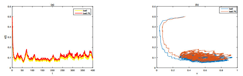
This paper presents long-time analysis of a stochastic chemostat model with instantaneous nutrient recycling. We focus on the investigation of the sufficient and almost necessary conditions of the exponential extinction and persistence for the model. The convergence to the invariant measure is also established under total variation norm. Our work generalizes and improves many existing results. One of the interesting findings is that random disturbance can suppress microorganism growth, which can provide us some useful control strategies to microbiological cultivation. Finally, some numerical simulations partly based on the stochastic sensitive function technique are given to illustrate theoretical results.
- stochastic chemostat model,
- extinction,
- persistence,
- ergodicity
Citation: Xiaoxia Guo, Dehao Ruan. Long-time analysis of a stochastic chemostat model with instantaneous nutrient recycling[J]. AIMS Mathematics, 2023, 8(4): 9331-9351. doi: 10.3934/math.2023469

Related Papers:

Abstract

This paper presents long-time analysis of a stochastic chemostat model with instantaneous nutrient recycling. We focus on the investigation of the sufficient and almost necessary conditions of the exponential extinction and persistence for the model. The convergence to the invariant measure is also established under total variation norm. Our work generalizes and improves many existing results. One of the interesting findings is that random disturbance can suppress microorganism growth, which can provide us some useful control strategies to microbiological cultivation. Finally, some numerical simulations partly based on the stochastic sensitive function technique are given to illustrate theoretical results.

References

[1]	L. Becks, F. M. Hilker, H. Malchow, K. Jürgens, H. Arndt, Experimental demonstration of chaos in a microbial food web, Nature, 435 (2005), 1226–1229. https://doi.org/10.1038/nature03627 doi: 10.1038/nature03627
[2]	A. Novick, L. Szilard, Description of the chemostat, Science, 112 (1950), 715–716. https://doi.org/10.1126/science.112.2920.715 doi: 10.1126/science.112.2920.715
[3]	A. W. Bush, A. E. Cool, The effect of time delay and growth rate inhibition in the bacterial treatment of wastewater, J. Theor. Biol., 63 (1976), 385–395. https://doi.org/10.1016/0022-5193(76)90041-2 doi: 10.1016/0022-5193(76)90041-2
[4]	S. Ruan, S. K. Wolkowicz, Bifurcation analysis of a chemostat model with a distributed delay, J. Math. Anal. Appl., 204 (1996), 786–812. https://doi.org/10.1006/jmaa.1996.0468 doi: 10.1006/jmaa.1996.0468
[5]	X. Meng, Q. Zhao, L. Chen, Global qualitative analysis of new Monod type chemostat model with delayed growth response and pulsed input in polluted environment, Appl. Math. Mech., 29 (2008), 75–87. https://doi.org/10.1007/s10483-008-0110-x doi: 10.1007/s10483-008-0110-x
[6]	M. Rehim, L. L. Sun, X. Abdurahman, Z. D. Teng, Study of chemostat model with impulsive input and nutrient recycling in a environment, Commun. Nonlinear Sci., 16 (2011), 2563–2574. https://doi.org/10.1016/j.cnsns.2010.09.030 doi: 10.1016/j.cnsns.2010.09.030
[7]	G. Pang, F. Wang, L. Chen, Study of Lotka-volterra food chain chemostat with periodically varying dilution rate, J. Math. Chem., 43 (2008), 901–913. https://doi.org/10.1007/s10910-007-9263-5 doi: 10.1007/s10910-007-9263-5
[8]	T. Wang, L. Chen, Global analysis of a three-dimensional delayed Michaelis-Menten chemostat-type models with pulsed input, J. Appl. Math. Comput., 35 (2011), 211–227. https://doi.org/10.1007/s12190-009-0352-4 doi: 10.1007/s12190-009-0352-4
[9]	G. Pang, F. Wang, L. Chen, Analysis of a Monod-Haldene type food chain chemostat with periodically varying substrate, Chaos Soliton. Fract., 38 (2008), 731–742. https://doi.org/10.1016/j.chaos.2007.01.018 doi: 10.1016/j.chaos.2007.01.018
[10]	G. J. Butler, G. S. K. Wolkowicz, A mathematical model of the chemostat with a general class of functions describing nutrient uptake, SIAM J. Appl. Math., 45 (1985), 138–151. https://doi.org/10.1137/0145006 doi: 10.1137/0145006
[11]	F. Campillo, M. Joannides, I. Larramendy-Valverde, Stochastic modeling of the chemostat, Ecol. Model., 222 (2011), 2676–2689. https://doi.org/10.1016/j.ecolmodel.2011.04.027 doi: 10.1016/j.ecolmodel.2011.04.027
[12]	L. Imhof, S. Walcher, Exclusion and persistence in deterministic and stochastic chemostat models, J. Differ. Equ., 217 (2005), 26–53. https://doi.org/10.1016/j.jde.2005.06.017 doi: 10.1016/j.jde.2005.06.017
[13]	H. J. Alsakaji, F. A. Rihan, A. Hashish, Dynamics of a tsochastic epidemic model with vaccination and multiple time-delays for COVID-19 in the UAE, Complexity, 2022 (2022), 4247800. https://doi.org/10.1155/2022/4247800 doi: 10.1155/2022/4247800
[14]	H. J. Alsakaji, F. A. Rihan, Stochastic delay differential equations of three-species prey-predator system with cooperation among prey species, Discrete Contin. Dyn. Syst., 15 (2022), 245–263. https://doi.org/10.3934/dcdss.2020468 doi: 10.3934/dcdss.2020468
[15]	X. Meng, L. Wang, T. Zhang, Global dynamics analysis of a nonlinear impulsive stochastic chemostat system in a polluted environment, J. Appl. Anal. Comput., 6 (2016), 865–875. https://doi.org/10.11948/2016055 doi: 10.11948/2016055
[16]	S. Sun, Y. Sun, G. Zhang, X. Liu, Dynamical behavior of a stochastic two-species Monod competition chemostat model, Appl. Math. Comput., 298 (2017), 153–170. https://doi.org/10.1016/j.amc.2016.11.005 doi: 10.1016/j.amc.2016.11.005
[17]	X. Lv, X. Meng, X. Wang, Extinction and stationary distribution of an impulsive stochastic chemostat model with nonlinear perturbation, Chaos Soliton. Fract., 110 (2018), 273–279. https://doi.org/10.1016/j.chaos.2018.03.038 doi: 10.1016/j.chaos.2018.03.038
[18]	D. H. Nguyen, N. Nguyen, G. Yin, General nonlinear stochastic systems motivated by chemostat models: Complete characterization of long-time behavior, optimal controls, and applications to wastewater treatment, Stoch. Proc. Appl., 130 (2020), 4608–4642. https://doi.org/10.1016/j.spa.2020.01.010 doi: 10.1016/j.spa.2020.01.010
[19]	J. Yang, Z. Zhao, X. Song, Statistical property analysis for a stochastic chemostat model with degenerate diffusion, AIMS Mathematics, 8 (2023), 1757–1769. https://doi.org/10.3934/math.2023090 doi: 10.3934/math.2023090
[20]	R. Baratti, J. Alvarez, S. Tronci, M. Grosso, A. Schaum, Characterization with Fokker-Planck theory of the nonlinear stochastic dynamics of a class of two-state continuous bioreactors, J. Process Contr., 102 (2021), 66–84. https://doi.org/10.1016/j.jprocont.2021.04.004 doi: 10.1016/j.jprocont.2021.04.004
[21]	A. Schaum, S. Tronci, R. Baratti, J. Alvarez, On the dynamics and robustness of the chemostat with multiplicative noise, IFAC-PapersOnLine, 54 (2021), 342–347. https://doi.org/10.1016/j.ifacol.2021.08.265 doi: 10.1016/j.ifacol.2021.08.265
[22]	X. Zhang, R. Yuan, The existence of stationary distribution of a stochastic delayed chemostat model, Appl. Math. Lett., 93 (2019), 15–21. https://doi.org/10.1016/j.aml.2019.01.034 doi: 10.1016/j.aml.2019.01.034
[23]	X. Zhang, R. Yuan, Stochastic properties of solution for a chemostat model with a distributed delay and random disturbance, Int. J. Biomath., 13 (2020), 2050065. https://doi.org/10.1142/s1793524520500667 doi: 10.1142/s1793524520500667
[24]	S. Sun, X. Zhang, Asymptotic behavior of a stochastic delayed chemostat model with nutrient storage, J. Biol. Syst., 26 (2018), 225–246. https://doi.org/10.1142/S0218339018500110 doi: 10.1142/S0218339018500110
[25]	F. Mazenc, S. L. Niculescu, G. Robledo, Stability analysis of mathematical model of competition in a chain of chemostats in series with delay, Appl. Math. Model., 76 (2019), 311–329. https://doi.org/10.1016/j.apm.2019.06.006 doi: 10.1016/j.apm.2019.06.006
[26]	W. Wang, W. Chen, Persistence and extinction of Markov switched stochastic Nicholson's blowies delayed differential equation, Int. J. Biomath., 13 (2020), 2050015. https://doi.org/10.1142/S1793524520500151 doi: 10.1142/S1793524520500151
[27]	G. Stephanopoulos, R. Aris, A. G. Fredrickson, A stochastic analysis of the growth of competing microbial populations in a continuous biochemical reactor, Math. Biosci., 45 (1979), 99–135. https://doi.org/10.1016/0025-5564(79)90098-1 doi: 10.1016/0025-5564(79)90098-1
[28]	L. Wang, D. Jiang, A note on the stationary distribution of the stochastic chemostat model with general response functions, Appl. Math. Lett., 73 (2017), 22–28. https://doi.org/10.1016/j.aml.2017.04.029 doi: 10.1016/j.aml.2017.04.029
[29]	R. M. Nisbet, W. Gurney, Model of material cycling in a closed ecosystem, Nature, 264 (1976), 633–634. https://doi.org/10.1038/264633a0 doi: 10.1038/264633a0
[30]	S. Ruan, Persistence and coexistence in zooplankton-phytoplankton-nutrient models with instantaneous nutrient recycling, J. Math. Biol., 31 (1993), 633–654. https://doi.org/10.1007/BF00161202 doi: 10.1007/BF00161202
[31]	Y. M. Svirezhev, D. O. Logofet, Stability of Biological Communities, Mir Publishers, 1983.
[32]	N. H. Du, N. H. Dang, N. T. Dieu, On stability in distribution of stochastic diferential delay equations with markovian switching, Syst. Control Lett., 65 (2014), 43–49. https://doi.org/10.1016/j.sysconle.2013.12.006 doi: 10.1016/j.sysconle.2013.12.006
[33]	N. T. Dieu, T. Fugo, N. H. Du, Asymptotic behaviors of stochastic epidemic models with jump-diffusion, Appl. Math. Model., 86 (2020), 259–270. https://doi.org/10.1016/j.apm.2020.05.003 doi: 10.1016/j.apm.2020.05.003
[34]	N. H. Du, N. N. Nhu, Permanence and extinction for the stochastic SIR epidemic model, J. Differ. Equ., 269 (2020), 9619–9652. https://doi.org/10.1016/j.jde.2020.06.049 doi: 10.1016/j.jde.2020.06.049
[35]	W. Kliemann, Recurrence and invariant measures for degenerate diffusions, Ann. Probab., 15 (1987), 690–707. https://doi.org/10.1214/aop/1176992166 doi: 10.1214/aop/1176992166
[36]	D. J. Higham, An algorithmic introduction to numerical simulation of stochastic differential equations, SIAM Rev., 43 (2001), 525–546. https://doi.org/10.1137/s0036144500378302 doi: 10.1137/s0036144500378302
[37]	L. B. Ryashko, I. A. Bashkirtseva, On control of stochastic sensitivity, Automat. Rem. Contr., 69 (2008), 1171–1180. https://doi.org/10.1134/S0005117908070084 doi: 10.1134/S0005117908070084

Reader Comments

Your name:*

Email:*
© 2023 the Author(s), licensee AIMS Press. This is an open access article distributed under the terms of the Creative Commons Attribution License (http://creativecommons.org/licenses/by/4.0)