Dynamical behavior of a stochastic predator-prey model with Holling-type III functional response and infectious predator

Chuangliang Qin; Jinji Du; Yuanxian Hui; Chuangliang Qin; Jinji Du; Yuanxian Hui

doi:10.3934/math.2022413

AIMS Mathematics

2022, Volume 7, Issue 5: 7403-7418. doi: 10.3934/math.2022413

Previous Article Next Article

Research article Special Issues

Dynamical behavior of a stochastic predator-prey model with Holling-type III functional response and infectious predator

1.
School of Mathematics and Statistics, Xinyang College, Xinyang 464000, China
2.
School of Mathematics and Statistics, Huanghuai University, Zhumadian 463000, China

Received: 17 November 2021 Revised: 12 January 2022 Accepted: 25 January 2022 Published: 11 February 2022
MSC : 34K20, 34D05, 92B05, 92D25

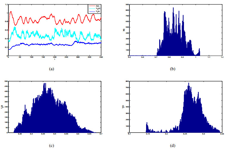
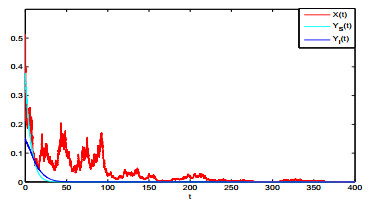
In this paper, we formulate a stochastic predator-prey model with Holling III type functional response and infectious predator. By constructing Lyapunov functions, we prove the global existence and uniqueness of the positive solution of the model, and establish the ergodic stationary distribution of the positive solution, which indicates that both the prey and predator will coexist for a long time. We also obtain sufficient conditions for the extinction of the predator and prey population. We finally provide numerical simulations to demonstrate our main results.
- stochastic predator-prey model,
- stationary distribution and ergodicity,
- extinction,
- Holling-type III functional response
Citation: Chuangliang Qin, Jinji Du, Yuanxian Hui. Dynamical behavior of a stochastic predator-prey model with Holling-type III functional response and infectious predator[J]. AIMS Mathematics, 2022, 7(5): 7403-7418. doi: 10.3934/math.2022413

Related Papers:

Abstract

In this paper, we formulate a stochastic predator-prey model with Holling III type functional response and infectious predator. By constructing Lyapunov functions, we prove the global existence and uniqueness of the positive solution of the model, and establish the ergodic stationary distribution of the positive solution, which indicates that both the prey and predator will coexist for a long time. We also obtain sufficient conditions for the extinction of the predator and prey population. We finally provide numerical simulations to demonstrate our main results.

References

[1]	A. J. Lotka, Elements of physical biology, Williams and Wilkins, 1925.
[2]	V. Volterra, Fluctuations in the abundance of a species considered mathematically, Nature, 118 (1926), 558–560. https://doi.org/10.1038/118558a0 doi: 10.1038/118558a0
[3]	R. A. Saenz, H. W. Hethcote, Competing species models with an infectious disease, Math. Biosci. Eng., 4 (2006), 219–235. https://doi.org/10.3934/mbe.2006.3.219 doi: 10.3934/mbe.2006.3.219
[4]	D. Barman, J. Roy, S. Alam, Dynamical behaviour of an infected predator-prey model with fear effect, Iran. J. Sci. Technol. A, 45 (2021), 309–325. https://doi.org/10.1007/s40995-020-01014-y doi: 10.1007/s40995-020-01014-y
[5]	A. Muh, A. Siddik, S. Toaha, A. M. Anwar, Stability analysis of prey-predator model with Holling type IV functional response and infectious predator, J. Mat. Stat. Komputasi, 17 (2021), 155–165. https://doi.org/10.20956/jmsk.v17i2.11716 doi: 10.20956/jmsk.v17i2.11716
[6]	S. X. Wu, X. Y. Meng, Dynamics of a delayed predator-prey system with fear effect, herd behavior and disease in the susceptible prey, AIMS Math., 6 (2021), 3654–3685. https://doi.org/10.3934/math.2021218 doi: 10.3934/math.2021218
[7]	W. Y. Shi, Y. L. Huang, C. J. Wei, S. W. Zhang, A stochastic Holling-type II predator-prey model with stage structure and refuge for prey, Adv. Math. Phys., 2021, 1–14. https://doi.org/10.1155/2021/9479012
[8]	Q. Liu, D. Q. Jiang, T. Hayat, Dynamics of stochastic predator-prey models with distributed delay and stage structure for prey, Int. J. Biomath., 14 (2021), 1–36.
[9]	T. T. Ma, X. Z. Meng, Z. B. Chang, Dynamics and optimal harvesting control for a stochastic one-predator-two-prey time delay system with jumps, Complexity, 2019, 1–19. https://doi.org/10.1155/2019/5342031
[10]	Q. Liu, D. Q. Jiang, Influence of the fear factor on the dynamics of a stochastic predator-prey mode, Appl. Math. Lett., 112 (2021), 106756. https://doi.org/10.1016/j.aml.2020.106756 doi: 10.1016/j.aml.2020.106756
[11]	H. K. Qi, X. Z. Meng, Threshold behavior of a stochastic predator-prey system with prey refuge and fear effect, Appl. Math. Lett., 113 (2021), 106846. https://doi.org/10.1016/j.aml.2020.106846 doi: 10.1016/j.aml.2020.106846
[12]	X. Mao, G. Marion, E. Renshaw, Environmental Brownian noise suppresses explosion in population dynamics, Stoch. Proc. Appl., 97 (2002), 95–110. https://doi.org/10.1016/S0304-4149(01)00126-0 doi: 10.1016/S0304-4149(01)00126-0
[13]	X. R. Mao, Stochastic differential equations and applications, Horwood Publishing, Chichester, 2007.
[14]	B. $\emptyset$ksendal, Stochastic differential equations: An introduction with applications, 5th edition, Universitext, Springer, Berlin, Germany, 1998. https://doi.org/10.1007/978-3-662-03620-4_1
[15]	R. Khsaminskii, Stochastic stability of differential equations, Heidelberg: Spinger-Verlag, 2012.
[16]	D. Higham, An algorithmic introduction to numerical simulation of stochastic differential equations, SIAM Rev., 43 (2001), 525–546. https://doi.org/10.1137/S0036144500378302 doi: 10.1137/S0036144500378302
[17]	F. A. Rihan, H. J. Alsakaji, Analysis of a stochastic HBV infection model with delayed immune response, Math. Biosci. Eng., 18 (2021), 5194–5220. https://doi.org/10.3934/mbe.2021264 doi: 10.3934/mbe.2021264
[18]	F. A. Rihan, H. J. Alsakaji, Stochastic delay differential equations of three-species prey-predator system with cooperation among prey species, Discrete Cont. Dyn.-S, 14 (2020), 1–20. https://doi.org/10.1186/s13662-020-02579-z doi: 10.1186/s13662-020-02579-z

Reader Comments

Your name:*

Email:*
© 2022 the Author(s), licensee AIMS Press. This is an open access article distributed under the terms of the Creative Commons Attribution License (http://creativecommons.org/licenses/by/4.0)