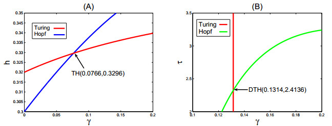
In this paper, under homogeneous Neumann boundary conditions, the complex dynamical behaviors of a diffusive Leslie-Gower predator-prey model with a ratio-dependent Holling type III functional response and nonlinear prey harvesting is carefully studied. By scrupulously analyzing and comprehending the distribution of the eigenvalues, the existence and stability (balance) of the extinction and coexistence equilibrium states are determined, and the bifurcations exhibited by the system are investigated by a mathematical analysis. Additionally, based on the theoretical analysis and numerical simulation, (Harvesting rate-induced, Delay-induced), Turing-Hopf bifurcations points are derived. Our results show that delay and nonlinear prey harvesting rates can create spatially inhomogeneous periodic solutions.
Citation: Heping Jiang. Complex dynamics induced by harvesting rate and delay in a diffusive Leslie-Gower predator-prey model[J]. AIMS Mathematics, 2023, 8(9): 20718-20730. doi: 10.3934/math.20231056
In this paper, under homogeneous Neumann boundary conditions, the complex dynamical behaviors of a diffusive Leslie-Gower predator-prey model with a ratio-dependent Holling type III functional response and nonlinear prey harvesting is carefully studied. By scrupulously analyzing and comprehending the distribution of the eigenvalues, the existence and stability (balance) of the extinction and coexistence equilibrium states are determined, and the bifurcations exhibited by the system are investigated by a mathematical analysis. Additionally, based on the theoretical analysis and numerical simulation, (Harvesting rate-induced, Delay-induced), Turing-Hopf bifurcations points are derived. Our results show that delay and nonlinear prey harvesting rates can create spatially inhomogeneous periodic solutions.

| [1] |
V. Ajraldi, M. Pittavino, E. Venturino, Modeling herd behavior in population systems, Nonlinear Anal. Real. World Appl., 12 (2011), 2319–2333. https://doi.org/10.1016/j.nonrwa.2011.02.002 doi: 10.1016/j.nonrwa.2011.02.002

|
| [2] |
P. A. Braza, Predator-prey dynamics with square root functional responses, Nonlinear Anal. Real. World Appl., 13 (2012), 1837–1843. https://doi.org/10.1016/j.nonrwa.2011.12.014 doi: 10.1016/j.nonrwa.2011.12.014
|
| [3] |
S. Chen, J. Shi, Global attractivity of equilibrium in Gierer-Meinhardt system with activator production saturation and gene expression time delays, Nonlinear Anal. Real. World Appl., 14 (2013), 1871–1886. https://doi.org/10.1016/j.nonrwa.2012.12.004 doi: 10.1016/j.nonrwa.2012.12.004
|
| [4] |
R. Yang, C. Nie, D. Jin, Spatiotemporal dynamics induced by nonlocal competition in a diffusive predator-prey system with habitat complexity, Nonlinear Dyn., 110 (2022), 879–900. https://doi.org/10.1007/s11071-022-07625-x doi: 10.1007/s11071-022-07625-x
|
| [5] |
R. Yang, D. Jin, W. Wang, A diffusive predator-prey model with generalist predator and time delay, AIMS Math., 7 (2022), 4574–4591. http://dx.doi.org/10.3934/math.2022255 doi: 10.3934/math.2022255
|
| [6] | T. Faria, Normal forms and Hopf bifurcation for partial differential equations with delay, Trans. Amer. Math. Soc., 352 (2000), 2217–2238. |
| [7] |
T. Faria, Stability and bifurcation for a delayed predator-prey model and the effect of diffusion, J. Math. Anal. Appl., 254 (2001), 433–463. https://doi.org/10.1006/jmaa.2000.7182 doi: 10.1006/jmaa.2000.7182
|
| [8] |
F. Yi, J. Wei, J. Shi, Bifurcation and spatio-temporal patterns in a homogeneous diffusive predator-prey system, J. Differ. Equ., 246 (2009), 1944–1977. https://doi.org/10.1016/j.jde.2008.10.024 doi: 10.1016/j.jde.2008.10.024
|
| [9] |
S. Yuan, C. Xu, T. Zhang, Spatial dynamics in a predator-prey model with herd behavior, Chaos, 23 (2013), 0331023. https://doi.org/10.1063/1.4812724 doi: 10.1063/1.4812724
|
| [10] |
S. Ruan, On nonlinear dynamics of predator-prey models with discrete delay, Math. Model. Nat. Phenom., 4 (2009), 140–188. https://doi.org/10.1051/mmnp/20094207 doi: 10.1051/mmnp/20094207
|
| [11] |
Y. Song, X. F. Zou, Bifurcation analysis of a diffusive ratio-dependent predator-prey model, Nonlinear Dyn., 78 (2014), 49–70. https://doi.org/10.1007/s11071-014-1421-2 doi: 10.1007/s11071-014-1421-2
|
| [12] |
Y. Song, Y. Peng, X. Zou, Persistence, stability and Hopf bifurcation in a diffusive ratio-dependent predator-prey model with delay, Int. J. Bifurcat. Chaos, 24 (2014), 1450093. https://doi.org/10.1142/S021812741450093X doi: 10.1142/S021812741450093X
|
| [13] |
X. Tang, Y. Song, Stability, Hopf bifurcations and spatial patterns in a delayed diffusive predator-prey model with herd behavior, Appl. Math. Comput., 254 (2015), 375–391. https://doi.org/10.1016/j.amc.2014.12.143 doi: 10.1016/j.amc.2014.12.143
|
| [14] |
R. M. May, J. R. Beddington, C. W. Clark, S. J. Holt, R. M. Laws, Management of multispecies fisheries, Science, 205 (1979), 267–277. https://doi.org/10.1126/science.205.4403.267 doi: 10.1126/science.205.4403.267
|
| [15] | R. P. Gupta, Malay Banerjee, Peeyush Chandra, Bifurcation analysis and control of Leslie-Gower predator-prey model with Michaelis-Menten type prey-harvesting, Differ. Equ. Dyn. Syst., 20, (2012) 339–366. https://doi.org/10.1007/s12591-012-0142-6 |
| [16] |
R. P. Gupta, Peeyush Chandra, Bifurcation analysis of modified Leslie-Gower predator-prey model with Michaelis-Menten type prey harvesting, J. Math. Anal. Appl., 398 (2013), 278–295. https://doi.org/10.1016/j.jmaa.2012.08.057 doi: 10.1016/j.jmaa.2012.08.057
|
| [17] |
R. P. Gupta, Peeyush Chandra, Malay Banerjee, Dynamical complexity of a predator-prey model with nonlinear predator harvesting, Discrete Contin. Dynam. Syst. Ser. B, 20 (2015), 423–443. http://dx.doi.org/10.3934/dcdsb.2015.20.423 doi: 10.3934/dcdsb.2015.20.423
|


Figures(3)

Heping Jiang. Complex dynamics induced by harvesting rate and delay in a diffusive Leslie-Gower predator-prey model[J]. AIMS Mathematics, 2023, 8(9): 20718-20730. doi: 10.3934/math.20231056


 DownLoad: