Numerical investigation for the fractional model of pollution for a system of lakes using the SCM based on the Appell type Changhee polynomials

Mohamed Adel; Mohamed M. Khader; Mohammed M. Babatin; Maged Z. Youssef; Mohamed Adel; Mohamed M. Khader; Mohammed M. Babatin; Maged Z. Youssef

doi:10.3934/math.20231592

AIMS Mathematics

2023, Volume 8, Issue 12: 31104-31117. doi: 10.3934/math.20231592

Previous Article Next Article

Research article Special Issues

Numerical investigation for the fractional model of pollution for a system of lakes using the SCM based on the Appell type Changhee polynomials

1.
Department of Mathematics, Faculty of Science, Islamic University of Madinah, Medina 42210, Saudi Arabia
2.
Department of Mathematics and Statistics, College of Science, Imam Mohammad, Ibn Saud Islamic University (IMSIU), Riyadh, 11566, Saudi Arabia
3.
Department of Mathematics, Faculty of Science, Benha University, Benha 13518, Egypt
4.
Department of Mathematics, Faculty of Science, Ain Shams University, Cairo 11566, Egypt

Received: 29 August 2023 Revised: 13 November 2023 Accepted: 15 November 2023 Published: 22 November 2023
MSC : 34A12, 41A30, 47H10, 65N20

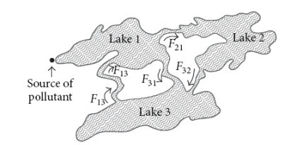
This article proposed a useful simulation to investigate the Liouville-Caputo fractional order pollution model's solution behavior for a network of three lakes connected by channels. A supposedly new approximation technique using the Appell type Changhee polynomials (ACPs) was used to treat the periodic and linear input models. This work employs the spectral collocation method based on the properties of the ACPs. The given technique creates a system of algebraic equations from the studied model. We verified the efficiency of the suggested technique by computing the residual error function. We compared the results to those obtained by the fourth-order Runge-Kutta method (RK4). Our findings confirmed that the technique used provides a straightforward and efficient tool to solve such problems. The key benefit of the suggested method is that it only requires a few easy steps, doesn't produce secular terms and doesn't rely on a perturbation parameter.
- model of pollution for system of lakes,
- Liouville-Caputo fractional derivative,
- APCs,
- spectral collocation method,
- fourth-order Runge-Kutta method
Citation: Mohamed Adel, Mohamed M. Khader, Mohammed M. Babatin, Maged Z. Youssef. Numerical investigation for the fractional model of pollution for a system of lakes using the SCM based on the Appell type Changhee polynomials[J]. AIMS Mathematics, 2023, 8(12): 31104-31117. doi: 10.3934/math.20231592

Related Papers:

Abstract

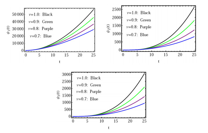
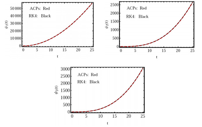
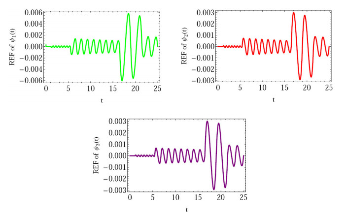
This article proposed a useful simulation to investigate the Liouville-Caputo fractional order pollution model's solution behavior for a network of three lakes connected by channels. A supposedly new approximation technique using the Appell type Changhee polynomials (ACPs) was used to treat the periodic and linear input models. This work employs the spectral collocation method based on the properties of the ACPs. The given technique creates a system of algebraic equations from the studied model. We verified the efficiency of the suggested technique by computing the residual error function. We compared the results to those obtained by the fourth-order Runge-Kutta method (RK4). Our findings confirmed that the technique used provides a straightforward and efficient tool to solve such problems. The key benefit of the suggested method is that it only requires a few easy steps, doesn't produce secular terms and doesn't rely on a perturbation parameter.

References

[1]	J. Biazar, M. Shahbala, H. Ebrahimi, VIM for solving the pollution problem of a system of lakes, J. Control Sci. Eng., 2010 (2010), 1–6. https://doi.org/10.1155/2010/829152 doi: 10.1155/2010/829152
[2]	J. Biazar, L. Farrokhi, M. R. Islam, Modeling the pollution of a system of lakes, Appl. Math. Comput., 178 (2006), 423–430. https://doi.org/10.1016/j.amc.2005.11.056 doi: 10.1016/j.amc.2005.11.056
[3]	M. Adel, M. M. Khader, S. Algelany, High-dimensional chaotic Lorenz system: Numerical treatment using Changhee polynomials of the Appell type, Fractal Fract., 7 (2023), 1–16. https://doi.org/10.3390/fractalfract7050398 doi: 10.3390/fractalfract7050398
[4]	Y. F. Ibrahim, S. E. Abd El-Bar, M. M. Khader, M. Adel, Studying and simulating the fractional COVID-19 model using an efficient spectral collocation approach, Fractal Fract., 7 (2023), 1–18. https://doi.org/10.3390/fractalfract7040307 doi: 10.3390/fractalfract7040307
[5]	M. Merdan, Homotopy perturbation method for solving modelling the pollution of a system of lakes, SDU J. Sci., 4 (2009), 99–111.
[6]	M. Merdan, A new application of modified differential transformation method for modelling the pollution of a system of lakes, Selcuk J. Appl. Math., 11 (2010), 27–40.
[7]	M. Merdan, He's variational iteration method for solving modelling the pollution of a system of lakes, Fen Bilimleri Dergisi, 18 (2009), 59–70.
[8]	Y. H. Youssri, W. M. Abd-Elhameed, Numerical spectral Legendre-Galerkin algorithm for solving time fractional telegraph equation, Rom. J. Phys., 63 (2018), 1–16.
[9]	M. M. Khader, K. M. Saad, A numerical study by using the Chebyshev collocation method for a problem of biological invasion: Fractional Fisher equation, Int. J. Biomath., 11 (2018), 1850099. https://doi.org/10.1142/S1793524518500997 doi: 10.1142/S1793524518500997
[10]	T. Patel, H. Patel, R. Meher, Analytical study of atmospheric internal waves model with fractional approach, J. Ocean Eng. Sci., 2022, In press. https://doi.org/10.1016/j.joes.2022.02.004
[11]	T. Patel, H. Patel, An analytical approach to solve the fractional-order (2+1)-dimensional Wu-Zhang equation, Math. Methods Appl. Sci., 46 (2023), 479–489. https://doi.org/10.1002/mma.8522 doi: 10.1002/mma.8522
[12]	H. Patel, T. Patel, D. Pandit, An efficient technique for solving fractional-order diffusion equations arising in oil pollution, J. Ocean Eng. Sci., 8 (2023), 217–225. https://doi.org/10.1016/j.joes.2022.01.004 doi: 10.1016/j.joes.2022.01.004
[13]	M. Alqhtani, M. M. Khader, K. M. Saad, Numerical simulation for a high-dimensional chaotic Lorenz system based on Gegenbauer wavelet polynomials, Mathematics, 11 (2023), 1–12. https://doi.org/10.3390/math11020472 doi: 10.3390/math11020472
[14]	A. A. Kilbas, H. M. Srivastava, J. J. Trujillo, Theory and applications of fractional differential equations, Elsevier, 2006.
[15]	H. M. Srivastava, An introductory overview of fractional-calculus operators based upon the Fox-Wright and related higher transcendental functions, J. Adv. Eng. Comput., 5 (2021), 135–166. http://dx.doi.org/10.55579/jaec.202153.340 doi: 10.55579/jaec.202153.340
[16]	D. S. Kim, T. Kim, J. J. Seo, A note on Changhee polynomials and numbers, Adv. Stud. Theor. Phys., 7 (2013), 993–1003.
[17]	J. G. Lee, L. C. Jang, J. J. Seo, S. K. Choi, H. I. Kwon, On Appell-type Changhee polynomials and numbers, Adv. Differ. Equ., 2016 (2016), 1–10. https://doi.org/10.1186/s13662-016-0866-7 doi: 10.1186/s13662-016-0866-7
[18]	S. Yuzbasi, N. Sahin, M. Sezer, A collocation approach to solving the model of pollution for a system of lakes, Math. Comput. Model., 55 (2012), 330–341. https://doi.org/10.1016/j.mcm.2011.08.007 doi: 10.1016/j.mcm.2011.08.007
[19]	J. C. Varekamp, Lake-pollution modelling, J. Geol. Educ., 36 (1988), 4–8. https://doi.org/10.5408/0022-1368-36.1.4 doi: 10.5408/0022-1368-36.1.4
[20]	B. Benhammouda, H. Vazquez-Leal, L. Hernandez-Martinez, Modified differential transform method for solving the model of pollution for a system of lakes, Discrete Dyn. Nat. Soc., 2014 (2014), 1–12. https://doi.org/10.1155/2014/645726 doi: 10.1155/2014/645726
[21]	E. U. Haq, Analytical solution of fractional model of pollution for a system lakes, Comput. Res. Prog. Appl. Sci. Eng., 6 (2020), 302–308.
[22]	M. Adel, M. M. Khader, Theoretical and numerical treatment for the fractal-fractional model of pollution for a system of lakes using an efficient numerical technique, Alex. Eng. J., 82 (2023), 415–425. https://doi.org/10.1016/j.aej.2023.10.003 doi: 10.1016/j.aej.2023.10.003
[23]	H. M. El-Hawary, M. S. Salim, H. S. Hussien, Ultraspherical integral method for optimal control problems governed by ordinary differential equations, J. Global Optim., 25 (2003), 283–303. https://doi.org/10.1023/A:1022463810376 doi: 10.1023/A:1022463810376

Reader Comments

Your name:*

Email:*
© 2023 the Author(s), licensee AIMS Press. This is an open access article distributed under the terms of the Creative Commons Attribution License (http://creativecommons.org/licenses/by/4.0)