Investigation of chaos behavior and integral sliding mode control on financial risk model

Sukono; Siti Hadiaty Yuningsih; Endang Rusyaman; Sundarapandian Vaidyanathan; Aceng Sambas; Sukono; Siti Hadiaty Yuningsih; Endang Rusyaman; Sundarapandian Vaidyanathan; Aceng Sambas

doi:10.3934/math.20221012

AIMS Mathematics

2022, Volume 7, Issue 10: 18377-18392. doi: 10.3934/math.20221012

Previous Article Next Article

Research article Special Issues

Investigation of chaos behavior and integral sliding mode control on financial risk model

1.
Department of Mathematics, Universitas Padjadjaran, Jatinangor, Kabupaten Sumedang 45363, Indonesia
2.
Magister Program of Mathematics, Universitas Padjadjaran, Jatinangor, Kabupaten Sumedang 45363, Indonesia
3.
Centre for Control Systems, Vel Tech University, Avadi, Chennai-600062, Tamil Nadu, India
4.
Department of Mechanical Engineering, Universitas Muhammadiyah Tasikmalaya, 46196, Indonesia
5.
Institute of Strategic Industrial Decision Modelling (ISIDM), Universiti Utara Malaysia, Sintok, Kedah 06010, Malaysia

Received: 13 March 2022 Revised: 27 July 2022 Accepted: 01 August 2022 Published: 16 August 2022
MSC : 34H10, 34K18, 34K20, 37G15

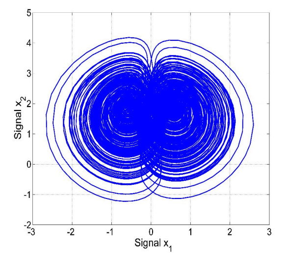
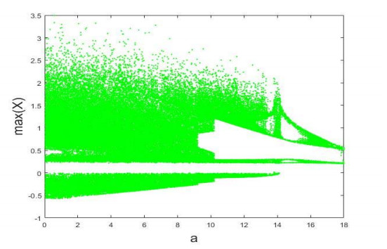
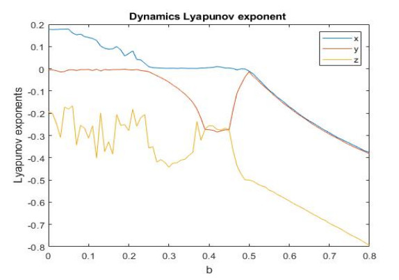
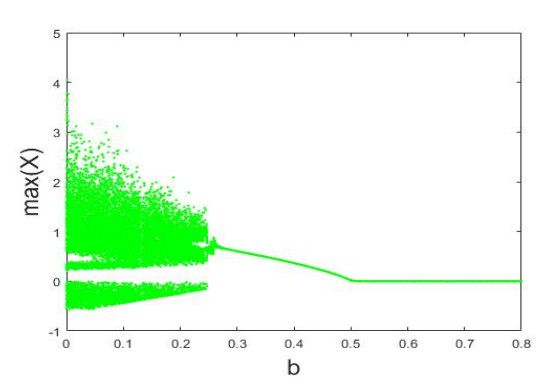
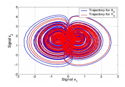
This paper reports the finding of a new financial chaotic system. A new control law for completely synchronizing the new financial chaotic system with itself has been established using adaptive integral sliding mode control. We also find that the new financial chaotic system has fascinating traits including symmetry, equilibrium points, multistability, Lyapunov exponents and bifurcation diagrams. We illustrate all the main results of this research work using MATLAB phase plots. The Lyapunov characteristic exponents and analysis using bifurcation diagrams have resulted in a new financial chaos system showing chaos phenomena in the intervals of parameters 0 < a < 15, and parameters 0 < b < 0.25. The results of this study can be used to predict if there is chaos in financial risk. Chaotic systems have many applications in engineering like cryptosystems and secure communication systems.
- chaos,
- financial chaotic system,
- integral sliding mode control,
- synchronization
Citation: Sukono, Siti Hadiaty Yuningsih, Endang Rusyaman, Sundarapandian Vaidyanathan, Aceng Sambas. Investigation of chaos behavior and integral sliding mode control on financial risk model[J]. AIMS Mathematics, 2022, 7(10): 18377-18392. doi: 10.3934/math.20221012

Related Papers:

Abstract

This paper reports the finding of a new financial chaotic system. A new control law for completely synchronizing the new financial chaotic system with itself has been established using adaptive integral sliding mode control. We also find that the new financial chaotic system has fascinating traits including symmetry, equilibrium points, multistability, Lyapunov exponents and bifurcation diagrams. We illustrate all the main results of this research work using MATLAB phase plots. The Lyapunov characteristic exponents and analysis using bifurcation diagrams have resulted in a new financial chaos system showing chaos phenomena in the intervals of parameters 0 < a < 15, and parameters 0 < b < 0.25. The results of this study can be used to predict if there is chaos in financial risk. Chaotic systems have many applications in engineering like cryptosystems and secure communication systems.

References

[1]	G. King, Restructuring the social sciences: Reflections from Harvard's institute for quantitative social science, Polit. Sci. Polit., 47 (2014), 165–172. https://doi.org/10.1017/S1049096513001534 doi: 10.1017/S1049096513001534
[2]	W. J. Baumol, B. Jess, Chaos: Significance, mechanism, and economic applications, J. Econ. Perspect., 3 (1989), 77–105. https://doi.org/10.1257/jep.3.1.77 doi: 10.1257/jep.3.1.77
[3]	H. Tirandaz, S. S. Aminabadi, H. Tavakoli, Chaos synchronization and parameter identification of a finance chaotic system with unknown parameters, a linear feedback controller, Alex. Eng. J., 57 (2018), 1519–1524. https://doi.org/10.1016/j.aej.2017.03.041 doi: 10.1016/j.aej.2017.03.041
[4]	K. Valaskova, T. Kliestik, L. Svabova, P. Adamko, Financial risk measurement and prediction modelling for sustainable development of business entities using regression analysis, Sustainability, 10 (2018). https://doi.org/10.3390/su10072144 doi: 10.3390/su10072144
[5]	J. D. Farmer, M. Gallegati, C. Hommes, A. Kirman, P. Ormerod, C. Cincotti, et al., A complex system approach to constructing better models for managing financial markets and the economy, Eur. Phys. J. Spec. Top., 214 (2012), 295–324. https://doi.org/10.1140/epjst/e2012-01696-9 doi: 10.1140/epjst/e2012-01696-9
[6]	A. T. Azar, S. Vaidyanathan, Computational intelligence applications in modeling and control, Springer: Berlin, Germany, 2014. https://doi.org/10.1007/978-3-319-11017-2
[7]	A. T. Azar, Chaos modeling and control system design, Springer: Berlin, Germany, 2015. https://doi.org/10.1007/978-3-319-13132-0
[8]	K. Tanaka, H. O. Wang, Fuzzy control system design and analysys, Wiley, 2001. https://doi.org/10.1002/0471224596
[9]	C. Wang, H. Zhang, W. Fan, et al., Adaptive control method for chaotic power systems based on finite-time stability theory and passivity-based control approach, Chaos Soliton. Fract., 112 (2018), 159–167. https://doi.org/10.1016/j.chaos.2018.05.005 doi: 10.1016/j.chaos.2018.05.005
[10]	F. Yu, L. Liu, H. Shen, Z. Zhang, Y. Huang, S. Cai, et al., Multistability analysis, coexisting multiple attractors, and FPGA implementation of Yu-Wang four-wing chaotic system, Math. Prob. Eng., 2020. https://doi.org/10.1155/2020/7530976 doi: 10.1155/2020/7530976
[11]	F. Yu, L. Liu, S. Qian, L. Li, Y. Huang, C. Shi, et al., Chaos-based application of a novel multistable 5D memristive hyperchaotic system with coexisting multiple Attractors, Complexity, 2020. https://doi.org/10.1155/2020/8034196 doi: 10.1155/2020/8034196
[12]	W. Wu, Z. Chen, Complex nonlinear dynamics and controlling chaos in a Cournot duopoly economic model, Nonlinear Anal.- Real, 11 (2010), 4363–4377. https://doi.org/10.1016/j.nonrwa.2010.05.022 doi: 10.1016/j.nonrwa.2010.05.022
[13]	W. T. Fitch, J. Neubauer, H. Herzel, Calls out of chaos: The adaptive significance of nonlinear phenomena in mammalian vocal production, Anim. Behav., 63 (2002), 407–418. https://doi.org/10.1006/anbe.2001.1912 doi: 10.1006/anbe.2001.1912
[14]	X. Ge, F. Yang, Q. L Han, Distributed networked control systems: A brief overview, Inform. Sci., 380 (2017), 117–131. https://doi.org/10.1016/j.ins.2015.07.047 doi: 10.1016/j.ins.2015.07.047
[15]	S. Vaidyanathan, Chaos in neurons and adaptive control of Birkhoff-Shaw strange chaotic attractor, Int. J. Pharm. Tech. Res., 8 (2015), 956–963.
[16]	A. Sambas, M. Mamat, A. A. Arafa, G. M. Mahmoud, Mohamed, M. S. W. A Sanjaya, A new chaotic system with line of equilibria: Dynamics, passive control and circuit design, Int. J. Electr. Comput., 9 (2019), 2365–2376. https://doi.org/10.11591/ijece.v9i4.pp2336-2345 doi: 10.11591/ijece.v9i4.pp2336-2345
[17]	S. Vaidyanathan, Adaptive control of a chemical chaotic reactor, Int. J. Pharm. Tech. Res., 8 (2015), 377–382.
[18]	S. Kumar, A. E. Matouk, H. Chaudhary, S. Kant, Control and synchronization of fractional-order chaotic satellite systems using feedback and adaptive control techniques, Int. J. Adapt. Control, 2020, 1–14. https://doi.org/10.1002/acs.3207 doi: 10.1002/acs.3207
[19]	I. Pan, S. Das, Fractional order fuzzy control of hybrid power system with renewable generation using chaotic PSO, ISA T., 62 (2016), 19–29. https://doi.org/10.1016/j.isatra.2015.03.003 doi: 10.1016/j.isatra.2015.03.003
[20]	Sukono, A. Sambas, S. He, H. Liu, J. Saputra, Dynamical analysis and adaptive fuzzy control for the fractional-order financial risk chaotic system, Adv. Differ. Equ., 674 (2020). https://doi.org/10.1186/s13662-020-03131-9 doi: 10.1186/s13662-020-03131-9
[21]	A. Bouzeriba, A. Boulkroune, T. Bouden, Projective synchronization of two different fractional-order chaotic systems via adaptive fuzzy control, Neural Comput. Appl., 27 (2016), 1349–1360. https://doi.org/10.1007/s00521-015-1938-4 doi: 10.1007/s00521-015-1938-4
[22]	M. T. Yassen, Chaos synchronization between two different chaotic systems using active control, Chaos Soliton. Fract., 23 (2005), 131–140. https://doi.org/10.1016/j.chaos.2004.03.038 doi: 10.1016/j.chaos.2004.03.038
[23]	E. W. Bai, K. E. Lonngren, Sequential synchronization of two Lorenz systems using active control, Chaos Soliton. Fract., 11 (2000), 1041–1044. https://doi.org/10.1016/S0960-0779(98)00328-2 doi: 10.1016/S0960-0779(98)00328-2
[24]	M. C. Ho, Y. C. Hung, Synchronization of two different systems by using generalized active control, Phys. Lett. A, 301 (2002), 424–428. https://doi.org/10.1016/S0375-9601(02)00987-8 doi: 10.1016/S0375-9601(02)00987-8
[25]	S. Vaidyanathan, S. Sampath, Anti-synchronization of four-wing chaotic systems via sliding mode control, Int. J. Autom. Comput., 9 (2012), 274–279. https://doi.org/10.1007/s11633-012-0644-2 doi: 10.1007/s11633-012-0644-2
[26]	Y. Pan, C. Yang, L. Pan, H. Yu, Integral sliding mode control: Performance, modification, and improvement, IEEE T. Ind. Inform., 14 (2018), 3087–3096. https://doi.org/10.1109/TII.2017.2761389 doi: 10.1109/TII.2017.2761389
[27]	N. Sene, Analysis of a four-dimensional hyperchaotic system described by the Caputo-Liouville fractional derivative, Complexity, 2020. https://doi.org/10.1155/2020/8889831 doi: 10.1155/2020/8889831
[28]	M. Diouf, N. Sene, Analysis of the financial chaotic model with the fractional derivative operator, Complexity, 2020. https://doi.org/10.1155/2020/9845031 doi: 10.1155/2020/9845031
[29]	S. Vaidyanathan, A. T. Azar, Hybrid synchronization of identical chaotic systems using sliding mode control and an application to Vaidyanathan chaotic systems, Stud. Comput. Intell., 576 (2015), 549–569. https://doi.org/10.1007/978-3-319-11173-5_20 doi: 10.1007/978-3-319-11173-5_20
[30]	A. Sambas, S. Vaidyanathan, Sudarno, M. Mamat, M. A. Mohamed, Investigation of chaos behavior in a new two-scroll chaotic system with four unstable equilibrium points, its synchronization via four control methods and circuit simulation, Int. J. Appl. Math., 50 (2020).
[31]	A. Sambas, Sukono, S. Vaidyanathan, Coexisting chaotic attractors and bifurcation analysis in a new chaotic system with close curve equilibrium points, Int. J. Adv. Sci. Tech., 29 (2020), 3329–3336.
[32]	N. Noroozi, B. Khaki, A. Sei, Chaotic oscillations damping in power system by nite time control theory, Int. Rev. Electr. Eng.-IREE, 3 (2008), 1032–1038.
[33]	Q. Gao, J. Ma, Chaos and Hopf bifurcation of a finance system, Nonlinear Dyn., 58 (2009), 209–216. https://doi.org/10.1007/s11071-009-9472-5 doi: 10.1007/s11071-009-9472-5
[34]	S. Vaidyanathan, C. K. Volos, O. I. Tacha, I. M. Kyprianidis, I. N. Stouboulos, V. T. Pham, Analysis, control and circuit simulation of a novel 3-D finance chaotic system, Stud. Comput. Intell., 536 (2016), 495–512. https://doi.org/10.1007/978-3-319-30279-9_21 doi: 10.1007/978-3-319-30279-9_21
[35]	O. I. Tacha, C. K. Volos, I. N. Stouboulos, I. M. Kyprianidis, Analysis, adaptive control and circuit simulation of a novel finance system with dissaving, Arch. Control Sci., 26 (2016), 95–115. https://doi.org/10.1515/acsc-2016-0006 doi: 10.1515/acsc-2016-0006
[36]	A. Sambas, S. Vaidyanathan, X. Zhang, I. Koyuncu, T. Bonny, M. Tuna, et al., A novel 3D chaotic system with line equilibrium: Multistability, integral sliding mode control, electronic circuit, FPGA and its image encryption, IEEE Access, 10 (2022), 2169–3536. https://doi.org/10.1109/ACCESS.2022.3181424 doi: 10.1109/ACCESS.2022.3181424
[37]	I. Yasser, A. T. Khalil, M. A. Mohamed, A. S. Samra, F. Khalifa, A robust chaos-based technique for medical image encryption, IEEE Access, 10 (2022), 244–257. https://doi.org/10.1109/ACCESS.2021.3138718 doi: 10.1109/ACCESS.2021.3138718
[38]	J. Zheng, H. Hu, A highly secure stream cipher based on analog-digital hybrid chaotic system, Inform. Sci., 587 (2022), 226–246. https://doi.org/10.1016/j.ins.2021.12.030 doi: 10.1016/j.ins.2021.12.030
[39]	F. Budiman, P. N. Andono, D. R. I. M. Setiadi, Image encryption using double layer chaos with dynamic iteration and rotation pattern, Int. J. Intell. Eng. Syst., 15 (2022), 57–67. https://doi.org/10.22266/ijies2022.0430.06 doi: 10.22266/ijies2022.0430.06
[40]	G. Arthi, V. Thanikaiselvan, R. Amirtharajan, 4D Hyperchaotic map and DNA encoding combined image encryption for secure communication, Multimed. Tools Appl., 81 (2022), 15859–15878. https://doi.org/10.1007/s11042-022-12598-5 doi: 10.1007/s11042-022-12598-5

Reader Comments

Your name:*

Email:*
© 2022 the Author(s), licensee AIMS Press. This is an open access article distributed under the terms of the Creative Commons Attribution License (http://creativecommons.org/licenses/by/4.0)