Pedal curves obtained from Frenet vector of a space curve and Smarandache curves belonging to these curves

Süleyman Şenyurt; Filiz Ertem Kaya; Davut Canlı; Süleyman Şenyurt; Filiz Ertem Kaya; Davut Canlı

doi:10.3934/math.2024981

AIMS Mathematics

2024, Volume 9, Issue 8: 20136-20162. doi: 10.3934/math.2024981

Previous Article Next Article

Research article

Pedal curves obtained from Frenet vector of a space curve and Smarandache curves belonging to these curves

1.
Department of Mathematics, Ordu University, Ordu, 52200, Türkiye
2.
Department of Mathematics, Niğde Ömer Halisdemir University, Niğde, 51240, Türkiye

Received: 02 May 2024 Revised: 05 June 2024 Accepted: 13 June 2024 Published: 20 June 2024
MSC : 53A04

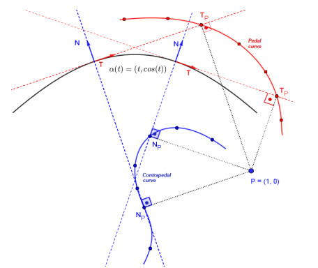
In this study, first the pedal curves as the geometric locus of perpendicular projections to the Frenet vectors of a space curve were defined and the Frenet vectors, curvature, and torsion of these pedal curves were calculated. Second, for each pedal curve, Smarandache curves were defined by taking the Frenet vectors as position vectors. Finally, the expressions of Frenet vectors, curvature, and torsion related to the main curves were obtained for each Smarandache curve. Thus, new curves were added to the curve family.

Keywords:

Citation: Süleyman Şenyurt, Filiz Ertem Kaya, Davut Canlı. Pedal curves obtained from Frenet vector of a space curve and Smarandache curves belonging to these curves[J]. AIMS Mathematics, 2024, 9(8): 20136-20162. doi: 10.3934/math.2024981

Related Papers:

[1]	Yanlin Li, A. A. Abdel-Salam, M. Khalifa Saad . Primitivoids of curves in Minkowski plane. AIMS Mathematics, 2023, 8(1): 2386-2406. doi: 10.3934/math.2023123
[2]	Semra Kaya Nurkan, İlkay Arslan Güven . Construction of vectorial moments via direction curves. AIMS Mathematics, 2023, 8(6): 12857-12871. doi: 10.3934/math.2023648
[3]	Esra Damar . Adjoint curves of special Smarandache curves with respect to Bishop frame. AIMS Mathematics, 2024, 9(12): 35355-35376. doi: 10.3934/math.20241680
[4]	Ayşe Yavuz, Melek Erdoǧdu . Non-lightlike Bertrand W curves: A new approach by system of differential equations for position vector. AIMS Mathematics, 2020, 5(6): 5422-5438. doi: 10.3934/math.2020348
[5]	Huina Zhang, Yanping Zhao, Jianguo Sun . The geometrical properties of the Smarandache curves on 3-dimension pseudo-spheres generated by null curves. AIMS Mathematics, 2024, 9(8): 21703-21730. doi: 10.3934/math.20241056
[6]	Sezai Kızıltuǧ, Tülay Erişir, Gökhan Mumcu, Yusuf Yaylı . $ C^* $-partner curves with modified adapted frame and their applications. AIMS Mathematics, 2023, 8(1): 1345-1359. doi: 10.3934/math.2023067
[7]	Muslum Aykut Akgun . Frenet curves in 3-dimensional $ \delta $-Lorentzian trans Sasakian manifolds. AIMS Mathematics, 2022, 7(1): 199-211. doi: 10.3934/math.2022012
[8]	Beyhan YILMAZ . Some curve pairs according to types of Bishop frame. AIMS Mathematics, 2021, 6(5): 4463-4473. doi: 10.3934/math.2021264
[9]	Ayman Elsharkawy, Ahmer Ali, Muhammad Hanif, Fatimah Alghamdi . Exploring quaternionic Bertrand curves: involutes and evolutes in $ \mathbb{E}^{4} $. AIMS Mathematics, 2025, 10(3): 4598-4619. doi: 10.3934/math.2025213
[10]	Ayman Elsharkawy, Clemente Cesarano, Abdelrhman Tawfiq, Abdul Aziz Ismail . The non-linear Schrödinger equation associated with the soliton surfaces in Minkowski 3-space. AIMS Mathematics, 2022, 7(10): 17879-17893. doi: 10.3934/math.2022985

Abstract

1. Introduction

The existence of curves in nature is a natural phenomenon that has been extensively studied by scientists. Researchers have formulated theories to understand the characteristics of these curves by careful examinations and valuable analysis. Therefore, the theory of curves has played a significant role in the field of differential geometry, making it an intriguing area of research.

To gain further insights and theoretical knowledge, it is the best practice to establish an orthonormal system on a curve. By doing so, scientists can gather more information and delve deeper into the properties of the curve. For instance, if the torsion of a curve is found to be zero, it indicates that the curve is planar, which concludes that if the torsion is nonzero, it signifies that the curve is a space curve. Moreover, the behavior of a curve can also be determined by examining its harmonic curvature defined as the ratio of the curvature to torsion. If the harmonic curvature function is constant, then the curve is classified as a helix. A Salkowski curve, on the other hand, is special due to its constant curvature and nonconstant torsion ^[1].

In addition, there exist other special paired curves possessing some mathematical relations between them. Examples of such pairs of curves include involute-evolute curves, Bertrand and Mannheim curves, as well as Successor curves and Smarandache curves. These curves have been extensively studied, contributing to a wealth of knowledge in this field ^[1,2,3,4,5].

Another interesting aspect of curve analysis involves the geometric location of perpendicular projection points onto the tangent or normal vector of a curve from a point that does not lie on the curve. This location is defined as the pedal (or contra-pedal) curve (see Figure 1).

Figure 1. The construction steps of pedal and contra-pedal curves for cosine function.

DownLoad: Full-Size Img PowerPoint

Extensive research has been conducted on these types of curves, and numerous sources provide valuable insights into their properties ^[6,7,8]. The study of such curves has been conducted using various frames in different spaces. Researchers have explored these curves using different approaches and continue to make significant contributions to this field of study ^{[9,10,11,12,13]}.

In this study, pedal curves belonging to the tangent, principal normal, and binormal vectors of a space curve are defined, and their Frenet vectors, curvature, and torsion functions are calculated. Next, Smarandache curves are defined by taking Frenet elements of each pedal curve as the position vectors. Finally, the corresponding Frenet apparatus are obtained and expressed in terms of the main curve. Thus, new curves are added to to the literature for the theory of curves. Let us recall the basic notions that will be used through the paper. For given a differentiable curve $\alpha(t)$ , the formulae of Frenet vector fields and curvature functions are defined as in the followings:

$\begin{align} T & = \frac{{\alpha '}}{{\left\| {\alpha '} \right\|}}, \quad N = B \wedge T = \frac{{\left( {\alpha ' \wedge \alpha ''} \right) \wedge \alpha '}}{{\left\| {\alpha ' \wedge \alpha ''} \right\|\left\| {\alpha '} \right\|}}, \quad B = \frac{{\alpha ' \wedge \alpha ''}}{{\left\| {\alpha ' \wedge \alpha ''} \right\|}}, \end{align}$

(1.1)

$\begin{align} \\ \kappa & = \frac{{\left\| {\alpha ' \wedge \alpha ''} \right\|}}{{{{\left\| {\alpha '} \right\|}^3}}}, \quad \tau = \frac{{\det \left( {\alpha ', \alpha '', \alpha '''} \right)}}{{{{\left\| {\alpha ' \wedge \alpha ''} \right\|}^2}}}, \end{align}$

(1.2)

$\begin{align} \\ T' & = v\kappa N, \quad N' = v\left( { - \kappa T + \tau B} \right), \quad B' = - v\tau N, \end{align}$

(1.3)

where $v = {\left\| {\alpha '} \right\|}$ , and " $\wedge$ " stands for the vector product operator ^[8,14].

Definition 1.1. Let $T_{\alpha}$ denote the tangent vector of a regular curve $\alpha$ in $\mathbb{E}^2$ . The geometric locus of the perpendicular projection of points onto a tangent vector from a given point $P \in \mathbb{E}^2$ that is not on the curve is called the pedal curve of the curve $\alpha$ ^[15].

Theorem 1.2. ^[15] The pedal curve of a regular curve $\alpha$ according to the point $P$ in $\mathbb{E}^2$ is given by the following equality:

$\begin{equation} {\alpha _P}\left( t \right) = \alpha \left( t \right) + \langle {P - \alpha \left( t \right), {T_\alpha }} \rangle {T_\alpha }. \end{equation}$

(1.4)

Definition 1.3. Let $N_{\alpha}$ be the normal vector of a regular curve $\alpha$ in $\mathbb{E}^2$ . The geometric locus of perpendicular projection of points onto the normal vector from a given point $P \in \mathbb{E}^2$ that is not on the curve is called the contra-pedal curve of the curve $\alpha$ ^[15].

Theorem 1.4. ^[15] The contra-pedal curve of a regular curve $\alpha$ according to the point $P$ in $\mathbb{E}^2$ is given by the following equality:

$\begin{equation} {\alpha ^ \bot }_P\left( t \right) = \alpha \left( t \right) + \langle {P - \alpha \left( t \right), {N_\alpha }} \rangle {N_\alpha }. \end{equation}$

(1.5)

Example 1.5. According to the origin $O(0, 0)$ , the pedal and contra-pedal curves of an ellipse that is parameterized as $\alpha(t) = (2cos(t), sin(t))$ in $\mathbb{E}^2$ is given by the following relations (see Figure 2).

${\alpha _P}\left( t \right) = \left( {\frac{{2\cos t}}{{1 + 3{{\sin }^2}t}}, \frac{{4\sin t}}{{1 + 3{{\sin }^2}t}}} \right), \qquad {\alpha ^ \bot }_P\left( t \right) = \left( {\frac{{7\cos t{{\sin }^2}t}}{{1 + 3{{\sin }^2}t}}, \frac{{3{{\sin }^3}t - \cos t\sin t}}{{1 + 3{{\sin }^2}t}}}\right) .$

Figure 2. The pedal (a) and contra-pedal (b) curves (red) of the ellipse (blue) according to the origin

$O(0, 0)$ where

$t \in [-\pi, \pi]$ .

DownLoad: Full-Size Img PowerPoint

2. T-Pedal curve and Smarandache curves of the T-Pedal curve

Definition 2.1. Let $T$ be the tangent vector of a given regular curve $\alpha$ in $\mathbb{E}^3$ . The geometric locus of the perpendicular projection of points onto a tangent vector from a point $P \in \mathbb{E}^3$ that is not on the curve is called the $T-pedal$ curve of the curve $\alpha$ according to $P$ .

Theorem 2.2. The equation of the $T-pedal$ curve of a given regular curve $\alpha$ is as follows:

$\begin{equation} {\alpha _T}\left( t \right) = \alpha \left( t \right) + \langle {P - \alpha \left( t \right), {T(t) }} \rangle {T(t)}. \end{equation}$

(2.1)

Proof. Let $P'$ be a perpendicular projection point onto the tangent vector from the point $P$ that is not on the curve $\alpha$ . The perpendicular projection vector $\overrightarrow {\alpha P'}$ is calculated by the following formula:

$\overrightarrow {\alpha P'} = \frac{{\langle {\alpha P, \alpha '} \rangle }}{{{{\left\| {\alpha '} \right\|}^2}}}\overrightarrow {\alpha '} .$

On the other hand, let $\alpha_T (t)$ be the geometric location of the point $P'$ . According to this, we obtain following equations:

$\begin{aligned} \overrightarrow {\alpha P} = \overrightarrow {\alpha P'} + \overrightarrow {P'P} & \Rightarrow \overrightarrow {\alpha P} = \frac{{\langle {\alpha P, \alpha '} \rangle }}{{{{\left\| {\alpha '} \right\|}^2}}}\overrightarrow {\alpha '} + \overrightarrow {P'P} \\ & \Rightarrow P' = \alpha + \frac{{\langle {P - \alpha , \alpha '} \rangle }}{{{{\left\| {\alpha '} \right\|}^2}}}\overrightarrow {\alpha '} \\ & \Rightarrow {\alpha _T}\left( t \right) = \alpha \left( t \right) + \langle {P - \alpha \left( t \right), \frac{{\alpha '}}{{\left\| {\alpha '} \right\|}}} \rangle \frac{{\alpha '}}{{\left\| {\alpha '} \right\|}}. \end{aligned}$

When the tangent vector from the relation (1.1) is taken into consideration, the proof of the theorem is completed. □

With some subsequent algebraic operations, if $u\left(t \right) = \langle {P - \alpha \left(t \right), T\left(t \right)} \rangle$ , then the relation (2.1) can be reduced to following:

$\begin{equation} {\alpha _T}\left( t \right) = \alpha \left( t \right) + u\left( t \right)T\left( t \right). \end{equation}$

(2.2)

Specifically, if the point $P$ is origin, then we have $u\left(t \right) = - \langle {\alpha \left(t \right), T\left(t \right)} \rangle$ .

Theorem 2.3. Let $\alpha_T$ be the $T-pedal$ curve of the given curve $\alpha$ with unit speed, and $\{T_1, \; N_1, \; B_1\}$ denotes the Frenet vectors of the $T-pedal$ curve of $\alpha$ . Then, among the Frenet vectors, the following relations exist:

$\begin{aligned} {T_1} = & {\omega _1}\left( {1 + u} \right)T + {\omega _1}u\kappa N, \\ {N_1} = & - {\eta _1}{\omega _1}u\kappa \left( {\kappa {{\left( {1 + u} \right)}^2} + {u^2}{\kappa ^3} + \left( {1 + u} \right){{\left( {u\kappa } \right)}^\prime } - uu'\kappa } \right)T\\ & + {\eta _1}{\omega _1}\left( {1 + u} \right)\left( {\kappa {{\left( {1 + u} \right)}^2} + {u^2}{\kappa ^3} + \left( {1 + u} \right){{\left( {u\kappa } \right)}^\prime } - uu'\kappa } \right)N\\ &+ \left( {{\eta _1}{\omega _1}\tau {{\left( {u\kappa } \right)}^3} + {\eta _1}{\omega _1}u\kappa \tau {{\left( {1 + u} \right)}^2}} \right)B, \\ {B_1} = & {\eta _1}\tau {\left( {u\kappa } \right)^2}T - {\eta _1}\left( {1 + u} \right)u\kappa \tau N + {\eta _1}\left( {\kappa {{\left( {1 + u} \right)}^2} + {u^2}{\kappa ^3} + \left( {1 + u} \right){{\left( {u\kappa } \right)}^\prime } - uu'\kappa } \right)B, \end{aligned}$

where

$\begin{aligned} {\omega _1} & = \frac{1}{{\sqrt {{{\left( {1 + u'} \right)}^2} + {{\left( {u\kappa } \right)}^2}} }}, \\ {\eta _1} & = \frac{1}{{\sqrt {{\tau ^2}{{\left( {u\kappa } \right)}^4} - {{\left( {1 + u'} \right)}^2}{{\left( {u\kappa \tau } \right)}^2} + {{\left( {{{\left( {1 + u'} \right)}^2}\kappa + \left( {1 + u'} \right){{\left( {u\kappa } \right)}^\prime } - u\kappa \left( {u'' - u{\kappa ^2}} \right)} \right)}^2}} }} \; . \end{aligned}$

Proof. By taking the necessary derivatives of the equality (2.2), we have

$\begin{align} {{\alpha '}_T} = & \left( {1 + u'} \right)T + u\kappa N, \\ {{\alpha ''}_T} = & \left( {u'' - u{\kappa ^2}} \right)T + \left( {\left( {1 + u'} \right)\kappa + {{\left( {u\kappa } \right)}^\prime }} \right)N + u\kappa \tau B, \\ {{\alpha '''}_T} = & \left( {u''' - {{\left( {u{\kappa ^2}} \right)}^\prime } - \left( {1 + u'} \right){\kappa ^2} - \kappa {{\left( {u\kappa } \right)}^\prime }} \right)T + \left( {u''\kappa - u{\kappa ^3} - u\kappa {\tau ^2} + {{\left( {\left( {1 + u'} \right)\kappa + {{\left( {u\kappa } \right)}^\prime }} \right)}^\prime }} \right)N \\ &+ \left( {\left( {1 + u'} \right)\tau \kappa + \tau {{\left( {u\kappa } \right)}^\prime } + {{\left( {u\kappa \tau } \right)}^\prime }} \right)B . \end{align}$

(2.3)

Upon necessary algebraic operations that are performed, the following relations are obtained

$\begin{align} {\alpha '_T} \wedge {\alpha ''_T} = & \tau {\left( {u\kappa } \right)^2}T - \left( {1 + u'} \right)u\kappa \tau N + \left( {{{\left( {1 + u'} \right)}^2}\kappa + \left( {1 + u'} \right){{\left( {u\kappa } \right)}^\prime } - u\kappa \left( {u'' - u{\kappa ^2}} \right)} \right)B, \\ \det \left( {{{\alpha '}_T}, {{\alpha ''}_T}, {{\alpha '''}_T}} \right) = & \tau {\left( {u\kappa } \right)^2}\left( {u''' - {{\left( {u{\kappa ^2}} \right)}^\prime } - \left( {1 + u'} \right){\kappa ^2} - \kappa {{\left( {u\kappa } \right)}^\prime }} \right)\\ & - u\kappa \tau \left( {1 + u'} \right)\left( {u''\kappa - u\kappa \left( {{\kappa ^2} + {\tau ^2}} \right) + {{\left( {\left( {1 + u'} \right)\kappa + {{\left( {u\kappa } \right)}^\prime }} \right)}^\prime }} \right) \\ & + \left( {{{\left( {1 + u'} \right)}^2}\kappa + \left( {1 + u'} \right){{\left( {u\kappa } \right)}^\prime } - u\kappa \left( {u'' - u{\kappa ^2}} \right)} \right)\left( {\left( {1 + u'} \right)\tau \kappa + \tau {{\left( {u\kappa } \right)}^\prime } + {{\left( {u\kappa \tau } \right)}^\prime }} \right), \end{align}$

(2.4)

$\begin{equation} \begin{aligned} \left\| {{{\alpha '}_T}} \right\| = & \sqrt {{{\left( {1 + u'} \right)}^2} + {{\left( {u\kappa } \right)}^2}} , \\ \left\| {{{\alpha '}_T} \wedge {{\alpha ''}_T}} \right\| = & \sqrt {{\tau ^2}{{\left( {u\kappa } \right)}^4} - {{\left( {1 + u'} \right)}^2}{{\left( {u\kappa \tau } \right)}^2} + {{\left( {{{\left( {1 + u'} \right)}^2}\kappa + \left( {1 + u'} \right){{\left( {u\kappa } \right)}^\prime } - u\kappa \left( {u'' - u{\kappa ^2}} \right)} \right)}^2}} \; \cdot \end{aligned} \end{equation}$

(2.5)

By substituting the given equalities above into the relations at (1.1), the proof is completed. □

Theorem 2.4. Let $\alpha_T$ be the $T-pedal$ curve of the unit speed curve $\alpha$ , and let $\kappa_1$ and $\tau_1$ denote the curvature and torsion functions for $\alpha_T$ , respectively. Then, the following relations exist among the curvatures:

$\begin{aligned} {\kappa _1} = & \frac{{{{\left( {{\tau ^2}{{\left( {u\kappa } \right)}^4} - {{\left( {1 + u'} \right)}^2}{{\left( {u\kappa \tau } \right)}^2} + {{\left( {{{\left( {1 + u'} \right)}^2}\kappa + \left( {1 + u'} \right){{\left( {u\kappa } \right)}^\prime } - u\kappa \left( {u'' - u{\kappa ^2}} \right)} \right)}^2}} \right)}^{\frac{1}{2}}}}}{{{{\left( {{{\left( {1 + u'} \right)}^2} + {{\left( {u\kappa } \right)}^2}} \right)}^{\frac{3}{2}}}}}, \\ {\tau _1} = & \frac{\begin{gathered} \tau {\left( {u\kappa } \right)^2}\left( {u''' - {{\left( {u{\kappa ^2}} \right)}^\prime } - \left( {1 + u'} \right){\kappa ^2} - \kappa {{\left( {u\kappa } \right)}^\prime }} \right) - u\kappa \tau \left( {1 + u'} \right)\left( {u''\kappa - u\kappa \left( {{\kappa ^2} + {\tau ^2}} \right) + {{\left( {\left( {1 + u'} \right)\kappa + {{\left( {u\kappa } \right)}^\prime }} \right)}^\prime }} \right) \hfill \\ + \left( {{{\left( {1 + u'} \right)}^2}\kappa + \left( {1 + u'} \right){{\left( {u\kappa } \right)}^\prime } - u\kappa \left( {u'' - u{\kappa ^2}} \right)} \right)\left( {\left( {1 + u'} \right)\tau \kappa + \tau {{\left( {u\kappa } \right)}^\prime } + {{\left( {u\kappa \tau } \right)}^\prime }} \right) \hfill \\ \end{gathered} }{{{\tau ^2}{{\left( {u\kappa } \right)}^4} - {{\left( {1 + u'} \right)}^2}{{\left( {u\kappa \tau } \right)}^2} + {{\left( {{{\left( {1 + u'} \right)}^2}\kappa + \left( {1 + u'} \right){{\left( {u\kappa } \right)}^\prime } - u\kappa \left( {u'' - u{\kappa ^2}} \right)} \right)}^2}}}. \end{aligned}$

Proof. By substituting the given relations (2.4) and (2.5) into (1.2), the curvatures can be found, completing the proof. □

Corollary 2.5. The following relations exist between the Frenet vectors of the $T-pedal$ curve and their derivatives

$\begin{equation} {T'_1} = {\mu _1}{\kappa _1}{N_1}, \qquad {N'_1} = {\mu _1}\left( { - {\kappa _1}{T_1} + {\tau _1}{B_1}} \right), \qquad {B'_1} = - {\mu _1}{\tau _1}{N_1}, \end{equation}$

(2.6)

where ${\mu _1} = \left\| {{{\alpha '}_T}} \right\|.$

Definition 2.6. By taking the tangent and the principal normal vectors of the $T-pedal$ curve as position vectors, we define a regular curve called the $T_1 N_1$ Smarandache curve as follows:

$\begin{equation} {\alpha _1} = \frac{{{T_1} + {N_1}}}{{\sqrt 2 }}. \end{equation}$

(2.7)

Theorem 2.7. Let $T_{\alpha _1}$ , $N_{\alpha _1}$ , and ${B_{{\alpha _1}}}$ be the Frenet vectors of the $T_1 N_1$ Smarandache curve. The relations among Frenet vectors are given as follows:

$\begin{align*} {T_{{\alpha _1}}} = & \frac{{ - {\kappa _1}{T_1} + {\kappa _1}{N_1} + {\tau _1}{B_1}}}{{\sqrt {2\kappa _1^2 + \tau _1^2} }} , \\ {N_{{\alpha _1}}} = & {B_{{\alpha _1}}} \wedge {T_{{\alpha _1}}}, \\ {B_{{\alpha _1}}} = & \frac{{ - \left( {{\kappa _1}{x_3} + {\tau _1}{x_2}} \right){T_1} + \left( {{\kappa _1}{x_3} + {\tau _1}{x_1}} \right){N_1} - \left( {{\kappa _1}{x_2} + {\kappa _1}{x_1}} \right){B_1}}}{{\sqrt {{{\left( {{\kappa _1}{x_3} + {\tau _1}{x_2}} \right)}^2} + {{\left( {{\kappa _1}{x_3} + {\tau _1}{x_1}} \right)}^2} + {{\left( {{\kappa _1}{x_2} + {\kappa _1}{x_1}} \right)}^2}} }}, \end{align*}$

where ${x_1} = - \frac{{\mu _1^2\kappa _1^2 - \left({{\mu _1}{\kappa _1}} \right)'}}{{\sqrt 2 }}, \; \; \; {\kern 1pt} {x_2} = \frac{{\left({{\mu _1}{\kappa _1}} \right)' - \mu _1^2\left({\kappa _1^2 + \tau _1^2} \right)}}{{\sqrt 2 }}, \; \; \; {\kern 1pt} {x_3} = \frac{{\mu _1^2{\kappa _1}{\tau _1} + \left({{\mu _1}{\tau _1}} \right)'}}{{\sqrt 2 }}.$

Proof. The derivatives of the $T_1 N_1$ curve up to the third degree are as given below.

$\begin{array}{l} {{\alpha '}_1} = \frac{{{\mu _1}\left( { - {\kappa _1}{T_1} + {\kappa _1}{N_1} + {\tau _1}{B_1}} \right)}}{{\sqrt 2 }}, \hfill \\ {{\alpha ''}_1} = {x_1}{T_1} + {x_2}{N_1} + {x_3}{B_1}, \hfill \\ {{\alpha '''}_1} = \left( {{{x'}_1} - {\mu _1}{\kappa _1}{x_2}} \right){T_1} + \left( {{{x'}_2} + {\mu _1}{x_1} - {\mu _1}{x_3}} \right){N_1} + \left( {{{x'}_3} + {\mu _1}{\tau _1}{x_2}} \right){B_1}. \end{array}$

(2.8)

By taking the vectoral product and computing the determinants of first and second derivatives of the curve $\alpha$ given in equality (2.8), we get the equality (2.9) as below:

$\begin{equation} \begin{aligned} {{\alpha '}_1} \wedge {{\alpha ''}_1} = & - \frac{{{\mu _1}\left( {{\kappa _1}{x_3} + {\tau _1}{x_2}} \right)}}{{\sqrt 2 }}{T_1} + \frac{{{\mu _1}\left( {{\kappa _1}{x_3} + {\tau _1}{x_1}} \right)}}{{\sqrt 2 }}{N_1} - \frac{{{\mu _1}\left( {{\kappa _1}{x_2} + {\kappa _1}{x_1}} \right)}}{{\sqrt 2 }}{B_1}, \hfill \\ \det \left( {{{\alpha '}_1}, {{\alpha ''}_1}, {{\alpha '''}_1}} \right) = & \frac{{{\mu _1}}}{{\sqrt 2 }}\left( \begin{array}{ll} \left( {{\kappa _1}{x_3} + {\tau _1}{x_1}} \right)\left( {{{x'}_2} + {\mu _1}{x_1} - {\mu _1}{x_3}} \right) - \left( {{\kappa _1}{x_3} + {\tau _1}{x_2}} \right)\left( {{{x'}_1} - {\mu _1}{\kappa _1}{x_2}} \right) \\ - \left( {{\kappa _1}{x_2} + {\kappa _1}{x_1}} \right)\left( {{{x'}_3} + {\mu _1}{\tau _1}{x_2}} \right) \\ \end{array} \right). \end{aligned} \end{equation}$

(2.9)

Moreover, by taking the norm of the first derivative of the curve $\alpha$ and the vectoral product of the first and second derivatives of $\alpha$ , we obtain the equality (2.10) as

$\begin{array}{l} \left\| {{{\alpha '}_1}} \right\| = \frac{{{\mu _1}}}{{\sqrt 2 }}\sqrt {2\kappa _1^2 + \tau _1^2} , \hfill \\ \left\| {{{\alpha '}_1} \wedge {{\alpha ''}_1}} \right\| = \frac{{{\mu _1}}}{{\sqrt 2 }}\sqrt {{{\left( {{\kappa _1}{x_3} + {\tau _1}{x_2}} \right)}^2} + {{\left( {{\kappa _1}{x_3} + {\tau _1}{x_1}} \right)}^2} + {{\left( {{\kappa _1}{x_2} + {\kappa _1}{x_1}} \right)}^2}} . \end{array}$

(2.10)

Finally, substituting the relations (2.8), (2.9), and (2.10) into (1.1) completes the proof. □

Theorem 2.8. Let $\kappa _{{\alpha _1}}$ and $\tau_{{\alpha _1}}$ denote the curvature and the torsion of the $T_1 N_1$ Smarandache curve, respectively. The following relations exist among the curvatures as

$\begin{aligned} {\kappa _{{\alpha _1}}} = & \frac{{2\sqrt {{{\left( {{\kappa _1}{x_3} + {\tau _1}{x_2}} \right)}^2} + {{\left( {{\kappa _1}{x_3} + {\tau _1}{x_1}} \right)}^2} + {{\left( {{\kappa _1}{x_2} + {\kappa _1}{x_1}} \right)}^2}} }}{{\mu _1^2\left( {2\kappa _1^2 + \tau _1^2} \right)\sqrt {2\kappa _1^2 + \tau _1^2} }}, \\ {\tau _{{\alpha _1}}} = & \frac{\begin{gathered} \sqrt 2 \left( {{\kappa _1}{x_3} + {\tau _1}{x_1}} \right)\left( {{{x'}_2} + {\mu _1}{x_1} - {\mu _1}{x_3}} \right) - \sqrt 2 \left( {{\kappa _1}{x_3} + {\tau _1}{x_2}} \right)\left( {{{x'}_1} - {\mu _1}{\kappa _1}{x_2}} \right) \hfill \\ - \sqrt 2 \left( {{\kappa _1}{x_2} + {\kappa _1}{x_1}} \right)\left( {{{x'}_3} + {\mu _1}{\tau _1}{x_2}} \right) \hfill \\ \end{gathered} }{{{\mu _1}{{\left( {{\kappa _1}{x_3} + {\tau _1}{x_2}} \right)}^2} + {\mu _1}{{\left( {{\kappa _1}{x_3} + {\tau _1}{x_1}} \right)}^2} + {\mu _1}{{\left( {{\kappa _1}{x_2} + {\kappa _1}{x_1}} \right)}^2}}}. \end{aligned}$

Proof. By using (2.9) and (2.10) to substitute into (1.2), the proof is completed. □

Definition 2.9. By taking the tangent and the binormal vectors of the $T-pedal$ curve as position vectors, we define a regular curve called the $T_1 B_1$ Smarandache curve as follows:

$\begin{equation} {\alpha _2} = \frac{{{T_1} + {B_1}}}{{\sqrt 2 }}. \end{equation}$

(2.11)

Theorem 2.10. Let ${T_{{\alpha _2}}}$ , ${N_{{\alpha _2}}}$ , and ${B_{{\alpha _2}}}$ be the Frenet vectors of the $T_1 B_1$ Smarandache curve. The relations among Frenet vectors are given as follows:

${T_{{\alpha _2}}} = {N_1}, \qquad {N_{{\alpha _2}}} = \frac{{ - {\kappa _1}{T_1} + {\tau _1}{B_1}}}{{\sqrt {\kappa _1^2 + \tau _1^2} }}, \qquad {B_{{\alpha _2}}} = \frac{{{\tau _1}{T_1} + {\kappa _1}{B_1}}}{{\sqrt {\kappa _1^2 + \tau _1^2} }}.$

Proof. By taking the derivatives of (2.11), we first have

$\begin{align} {{\alpha '}_2} = & \frac{{{\mu _1}\left( {{\kappa _1} - {\tau _1}} \right){N_1}}}{{\sqrt 2 }}, \\ {{\alpha ''}_2} = & \frac{{ - {\kappa _1}\mu _1^2\left( {{\kappa _1} - {\tau _1}} \right){T_1} + {{\left( {{\mu _1}{\kappa _1} - {\mu _1}{\tau _1}} \right)}^\prime }{N_1} + {\tau _1}\mu _1^2\left( {{\kappa _1} - {\tau _1}} \right){B_1}}}{{\sqrt 2 }}, \\ {{\alpha '''}_2} = &\frac{\begin{array}{ll} \left( {{{\left( { - {\kappa _1}\mu _1^2\left( {{\kappa _1} - {\tau _1}} \right)} \right)}^\prime } - {\kappa _1}{\mu _1}{{\left( {{\mu _1}{\kappa _1} - {\mu _1}{\tau _1}} \right)}^{\prime \prime }}} \right){T_1} + \left( {{{\left( {{\mu _1}{\kappa _1} - {\mu _1}{\tau _1}} \right)}^{\prime \prime }} - \mu _1^3\left( {{\kappa _1} - {\tau _1}} \right)\left( {\kappa _1^2 + \tau _1^2} \right)} \right){N_1} \\ + \left( {{{\left( {{\tau _1}\mu _1^2\left( {{\kappa _1} - {\tau _1}} \right)} \right)}^\prime } + {\tau _1}{\mu _1}{{\left( {{\mu _1}{\kappa _1} - {\mu _1}{\tau _1}} \right)}^{\prime \prime }}} \right){B_1} \\ \end{array} }{{\sqrt 2 }}. \end{align}$

(2.12)

Further, by taking norms and having required vector products, we have

$\begin{equation} \begin{aligned} {{\alpha '}_2} \wedge {{\alpha ''}_2} = & \frac{{\mu _1^3{{\left( {{\kappa _1} - {\tau _1}} \right)}^2}\left( {{\tau _1}{T_1} + {\kappa _1}{B_1}} \right)}}{2}, \\ \det \left( {{{\alpha '}_2}, {{\alpha ''}_2}, {{\alpha '''}_2}} \right) = & \frac{{\mu _1^5{{\left( {{\kappa _1} - {\tau _1}} \right)}^3}\left( {{\kappa _1}{\tau _1}' - {\kappa _1}'{\tau _1}} \right)}}{{2\sqrt 2 }}, \end{aligned} \end{equation}$

(2.13)

and

$\begin{equation} \left\| {{{\alpha '}_2}} \right\| = \frac{{{\mu _1}\left( {{\kappa _1} - {\tau _1}} \right)}}{{\sqrt 2 }}, \qquad \left\| {{{\alpha '}_2} \wedge {{\alpha ''}_2}} \right\| = \frac{{\mu _1^3{{\left( {{\kappa _1} - {\tau _1}} \right)}^2}\sqrt {\kappa _1^2 + \tau _1^2} }}{2}. \end{equation}$

(2.14)

If we substitute relations (2.12), (2.13), and (2.14) into (1.1), the proof is completed. □

Theorem 2.11. Let $\kappa _{{\alpha _2}}$ and $\tau_{{\alpha _2}}$ denote the curvature and the torsion of the $T_1 B_1$ Smarandache curve, respectively. The following relations exist among the curvatures as

${\kappa _{{\alpha _2}}} = \frac{{\sqrt {2\kappa _1^2 + 2\tau _1^2} }}{{\left( {{\kappa _1} - {\tau _1}} \right)}}, \qquad {\tau _{{\alpha _2}}} = \frac{{\sqrt 2 \left( {{\kappa _1}{\tau _1}' - {\kappa _1}'{\tau _1}} \right)}}{{{\mu _1}\left( {{\kappa _1} - {\tau _1}} \right)\left( {\kappa _1^2 + \tau _1^2} \right)}}.$

Proof. The proof is obvious by the substitution of (2.13) and (2.14) into (1.2). □

Definition 2.12. By taking the principal normal and the binormal vectors of the $T-pedal$ curve as position vectors, we define a regular curve called the $N_1 B_1$ Smarandache curve as follows:

$\begin{equation} {\alpha _3} = \frac{{{N_1} + {B_1}}}{{\sqrt 2 }}. \end{equation}$

(2.15)

Theorem 2.13. Let ${T_{{\alpha _3}}}$ , ${N_{{\alpha _3}}}$ , and ${B_{{\alpha _3}}}$ be the Frenet vectors of the $N_1 B_1$ Smarandache curve. The relations among Frenet vectors are given as follows:

$\begin{array}{l} {T_{{\alpha _3}}} = \frac{{ - {\kappa _1}{T_1} - {\tau _1}{N_1} + {\tau _1}{B_1}}}{{\sqrt {\kappa _1^2 + 2\tau _1^2} }}, \hfill \\ {N_{{\alpha _3}}} = {B_{{\alpha _3}}} \wedge {T_{{\alpha _3}}}, \hfill \\ {B_{{\alpha _3}}} = \frac{{ - \left( {{\tau _1}{y_3} + {\tau _1}{y_2}} \right){T_1} + \left( {{\kappa _1}{y_3} + {\tau _1}{y_1}} \right){N_1} + \left( {{\tau _1}{y_1} - {\kappa _1}{y_2}} \right){B_1}}}{{\sqrt {{{\left( {{\tau _1}{y_3} + {\tau _1}{y_2}} \right)}^2} + {{\left( {{\kappa _1}{y_3} + {\tau _1}{y_1}} \right)}^2} + {{\left( {{\tau _1}{y_1} - {\kappa _1}{y_2}} \right)}^2}} }}, \hfill \\ \end{array}$

where ${y_1} = \frac{{\mu _1^2{\tau _1}{\kappa _1} - {{\left({{\mu _1}{\kappa _1}} \right)}^\prime }}}{{\sqrt 2 }}, \quad {y_2} = - \frac{{\mu _1^2\left({\kappa _1^2 + \tau _1^2} \right) + {{\left({{\mu _1}{\tau _1}} \right)}^\prime }}}{{\sqrt 2 }}, \quad {y_3} = \frac{{{{\left({{\mu _1}{\tau _1}} \right)}^\prime } - \mu _1^2\tau _1^2}}{{\sqrt 2 }} \cdot$

Proof. By taking the derivatives of (2.15), we have

$\begin{equation} \begin{aligned} {{\alpha '}_3} = & \frac{{{\mu _1}\left( { - {\kappa _1}{T_1} - {\tau _1}{N_1} + {\tau _1}{B_1}} \right)}}{{\sqrt 2 }}, \\ {{\alpha ''}_3} = & {y_1}{T_1} + {y_2}{N_1} + {y_3}{B_1}, \\ {{\alpha '''}_3} = & \left( {{{y'}_1} - {\mu _1}{y_2}{\kappa _1}} \right){T_1} + \left( {{{y'}_2} + {\mu _1}{y_1}{\kappa _1} - {\mu _1}{y_3}{\tau _1}} \right){N_1} + \left( {{{y'}_3} + {\mu _1}{y_2}{\tau _1}} \right){B_1}. \\ \end{aligned} \end{equation}$

(2.16)

Moreover, we calculate the required vector products and the norms as

$\begin{equation} \begin{aligned} {{\alpha '}_3} \wedge {{\alpha ''}_3} = & \frac{{{\mu _1}}}{{\sqrt 2 }}\left( {\left( { - \left( {{\tau _1}{y_3} + {\tau _1}{y_2}} \right){T_1} + \left( {{\kappa _1}{y_3} + {\tau _1}{y_1}} \right){N_1} + \left( {{\tau _1}{y_1} - {\kappa _1}{y_2}} \right){B_1}} \right)} \right), \\ \det \left( {{{\alpha '}_3}, {{\alpha ''}_3}, {{\alpha '''}_3}} \right) = & \frac{{{\mu _1}}}{{\sqrt 2 }}\left( \begin{gathered} \left( {{\tau _1}{y_1} - {\kappa _1}{y_2}} \right)\left( {{{y'}_3} + {\mu _1}{y_2}{\tau _1}} \right) - \left( {{\tau _1}{y_3} + {\tau _1}{y_2}} \right)\left( {{{y'}_1} - {\mu _1}{y_2}{\kappa _1}} \right) \hfill \\ + \left( {{{y'}_1} - {\mu _1}{y_2}{\kappa _1}} \right)\left( {{{y'}_2} + {\mu _1}{y_1}{\kappa _1} - {\mu _1}{y_3}{\tau _1}} \right) \hfill \\ \end{gathered} \right) \end{aligned} \end{equation}$

(2.17)

and

$\begin{equation} \begin{aligned} \left\| {{{\alpha '}_3}} \right\| = & \frac{{{\mu _1}}}{{\sqrt 2 }}\sqrt {\kappa _1^2 + 2\tau _1^2} , \\ \left\| {{{\alpha '}_3} \wedge {{\alpha ''}_3}} \right\| = & \frac{{{\mu _1}}}{{\sqrt 2 }}\sqrt {{{\left( {{\tau _1}{y_3} + {\tau _1}{y_2}} \right)}^2} + {{\left( {{\kappa _1}{y_3} + {\tau _1}{y_1}} \right)}^2} + {{\left( {{\tau _1}{y_1} - {\kappa _1}{y_2}} \right)}^2}}. \end{aligned} \end{equation}$

(2.18)

When substituting relations (2.16), (2.17), and (2.18) into (1.1), the proof is completed. □

Theorem 2.14. Let $\kappa _{{\alpha _3}}$ and $\tau_{{\alpha _3}}$ denote the curvature and the torsion of the $T_1 B_1$ Smarandache curve, respectively. The following relations exist among the curvatures as

${\kappa _{{\alpha _3}}} = \frac{{2\sqrt {{{\left( {{\tau _1}{y_3} + {\tau _1}{y_2}} \right)}^2} + {{\left( {{\kappa _1}{y_3} + {\tau _1}{y_1}} \right)}^2} + {{\left( {{\tau _1}{y_1} - {\kappa _1}{y_2}} \right)}^2}} }}{{\mu _{^1}^2\left( {\kappa _1^2 + 2\tau _1^2} \right)\sqrt {\kappa _1^2 + 2\tau _1^2} }}, \\$

${\tau _{{\alpha _3}}} = \frac{{\sqrt 2 \left( \begin{gathered} \left( {{\tau _1}{y_1} - {\kappa _1}{y_2}} \right)\left( {{{y'}_3} + {\mu _1}{y_2}{\tau _1}} \right) - \left( {{\tau _1}{y_3} + {\tau _1}{y_2}} \right)\left( {{{y'}_1} - {\mu _1}{y_2}{\kappa _1}} \right) \\ + \left( {{{y'}_1} - {\mu _1}{y_2}{\kappa _1}} \right)\left( {{{y'}_2} + {\mu _1}{y_1}{\kappa _1} - {\mu _1}{y_3}{\tau _1}} \right) \\ \end{gathered} \right)}}{{{\mu _1}\left( {{{\left( {{\tau _1}{y_3} + {\tau _1}{y_2}} \right)}^2} + {{\left( {{\kappa _1}{y_3} + {\tau _1}{y_1}} \right)}^2} + {{\left( {{\tau _1}{y_1} - {\kappa _1}{y_2}} \right)}^2}} \right)}} .$

Proof. The proof is done upon substituting the above relations (2.17) and (2.18) into (1.2). □

Definition 2.15. By taking the tangent and principal normal and binormal vectors of the $T-pedal$ curve as position vectors, we define a regular curve called the $T_1 N_1 B_1$ Smarandache curve as follows:

$\begin{equation} {\alpha _4} = \frac{{{T_1}+{N_1} + {B_1}}}{{\sqrt 3 }}. \end{equation}$

(2.19)

Theorem 2.16. Let ${T_{{\alpha _4}}}$ , ${N_{{\alpha _4}}}$ , and ${B_{{\alpha _4}}}$ be the Frenet vectors of the $T_1 N_1 B_1$ Smarandache curve. The relations among Frenet vectors are given as follows:

$\begin{aligned} {T_{{\alpha _4}}} = & \frac{{ - {\kappa _1}{T_1} + \left( {{\kappa _1} - {\tau _1}} \right){N_1} + {\tau _1}{B_1}}}{{\sqrt {2\kappa _1^2 - 2{\kappa _1}{\tau _1} + 2\tau _1^2} }}, \\ {N_{{\alpha _4}}} = & {B_{{\alpha _4}}} \wedge {T_{{\alpha _4}}}, \\ {B_{{\alpha _4}}} = & \frac{{\left( {{z_3}{\kappa _1} - {z_3}{\tau _1} - {\tau _1}{z_2}} \right){T_1} + \left( {{\tau _1}{z_1} + {\kappa _1}{z_3}} \right){N_1} - \left( {{\kappa _1}{z_1} - {\tau _1}{z_1} + {\kappa _1}{z_2}} \right){B_1}}}{{\sqrt {{{\left( {{z_3}{\kappa _1} - {z_3}{\tau _1} - {\tau _1}{z_2}} \right)}^2} + {{\left( {{\tau _1}{z_1} + {\kappa _1}{z_3}} \right)}^2} + {{\left( {{\kappa _1}{z_1} - {\tau _1}{z_1} + {\kappa _1}{z_2}} \right)}^2}} }} \; , \end{aligned}$

where

$\begin{array}{ll} {z_1} = - \frac{{{{\left( {{\mu _1}{\kappa _1}} \right)}^\prime } + \mu _{^1}^2{\kappa _1}\left( {{\kappa _1} - {\tau _1}} \right)}}{{\sqrt 3 }}, \qquad {z_2} = \frac{{{{\left( {{\mu _1}{\kappa _1} - {\mu _1}{\tau _1}} \right)}^\prime } - \mu _{^1}^2\left( {\kappa _1^2 + \tau _1^2} \right)}}{{\sqrt 3 }}, \\ {z_3} = \frac{{{{\left( {{\mu _1}{\tau _1}} \right)}^\prime } + \mu _{^1}^2{\tau _1}\left( {{\kappa _1} - {\tau _1}} \right)}}{{\sqrt 3 }} \cdot \end{array}$

Proof. The derivatives of (2.19) are

$\begin{equation} \begin{aligned} {{\alpha '}_4} = & \frac{{{\mu _1}\left( { - {\kappa _1}{T_1} + \left( {{\kappa _1} - {\tau _1}} \right){N_1} + {\tau _1}{B_1}} \right)}}{{\sqrt 3 }}, \\ {{\alpha ''}_4} = & {z_1}{T_1} + {z_2}{N_1} + {z_3}{B_1}, \\ {{\alpha '''}_4} = & \left( {{{z'}_1} - {z_2}{\mu _1}{\kappa _1}} \right){T_1} + \left( {{{z'}_2} + {z_1}{\mu _1}{\kappa _1} - {z_3}{\mu _1}{\tau _1}} \right){N_1} + \left( {{{z'}_3} + {z_2}{\mu _1}{\tau _1}} \right){B_1}. \\ \end{aligned} \end{equation}$

(2.20)

In addition, the required vector products and the norms are calculated as

$\begin{equation} \begin{aligned} &{{\alpha '}_4} \wedge {{\alpha ''}_4} = \frac{{{\mu _1}}}{{\sqrt 3 }}\left( {\left( {{z_3}{\kappa _1} - {z_3}{\tau _1} - {\tau _1}{z_2}} \right){T_1} + \left( {{\tau _1}{z_1} + {\kappa _1}{z_3}} \right){N_1} - \left( {{\kappa _1}{z_1} - {\tau _1}{z_1} + {\kappa _1}{z_2}} \right){B_1}} \right), \\ &\det \left( {{{\alpha '}_4}, {{\alpha ''}_4}, {{\alpha '''}_4}} \right) = \frac{{{\mu _1}}}{{\sqrt 3 }}\left( \begin{array}{lll} \left( {{z_3}{\kappa _1} - {z_3}{\tau _1} - {\tau _1}{z_2}} \right)\left( {{{z'}_1} - {z_2}{\mu _1}{\kappa _1}} \right) \\ + \left( {{\tau _1}{z_1} + {\kappa _1}{z_3}} \right)\left( {{{z'}_2} + {z_1}{\mu _1}{\kappa _1} - {z_3}{\mu _1}{\tau _1}} \right) \\ - \left( {{\kappa _1}{z_1} - {\tau _1}{z_1} + {\kappa _1}{z_2}} \right)\left( {{{z'}_3} + {z_2}{\mu _1}{\tau _1}} \right) \end{array} \right) , \end{aligned} \end{equation}$

(2.21)

and

$\begin{equation} \begin{aligned} \left\| {{{\alpha '}_4}} \right\| = & \frac{{\sqrt 6 {\mu _1}}}{3}\sqrt {\kappa _1^2 - {\kappa _1}{\tau _1} + \tau _1^2} , \\ \left\| {{{\alpha '}_4} \wedge {{\alpha ''}_4}} \right\| = & \frac{{{\mu _1}}}{{\sqrt 3 }}\sqrt {{{\left( {{z_3}{\kappa _1} - {z_3}{\tau _1} - {\tau _1}{z_2}} \right)}^2} + {{\left( {{\tau _1}{z_1} + {\kappa _1}{z_3}} \right)}^2} + {{\left( {{\kappa _1}{z_1} - {\tau _1}{z_1} + {\kappa _1}{z_2}} \right)}^2}} \; \cdot \end{aligned} \end{equation}$

(2.22)

By substituting relations (2.20), (2.21), and (2.22) into (1.1), the proof is completed. □

Theorem 2.17. Let $\kappa _{{\alpha _4}}$ and $\tau_{{\alpha _4}}$ denote the curvature and the torsion of the $T_1 N_1 B_1$ Smarandache curve, respectively. The following relations exist among the curvatures as

$\begin{aligned} {\kappa _{{\alpha _4}}} = & \frac{{3\sqrt 2 }}{4} \frac{{\sqrt {{{\left( {{z_3}{\kappa _1} - {z_3}{\tau _1} - {\tau _1}{z_2}} \right)}^2} + {{\left( {{\tau _1}{z_1} + {\kappa _1}{z_3}} \right)}^2} + {{\left( {{\kappa _1}{z_1} - {\tau _1}{z_1} + {\kappa _1}{z_2}} \right)}^2}} }}{{\mu _1^2\left( {\kappa _1^2 - {\kappa _1}{\tau _1} + \tau _1^2} \right)\sqrt {\kappa _1^2 - {\kappa _1}{\tau _1} + \tau _1^2} }}, \\ {\tau _{{\alpha _4}}} = & \frac{{\sqrt 3 \left( \begin{array}{ll} \left( {{z_3}{\kappa _1} - {z_3}{\tau _1} - {\tau _1}{z_2}} \right)\left( {{{z'}_1} - {z_2}{\mu _1}{\kappa _1}} \right) + \left( {{\tau _1}{z_1} + {\kappa _1}{z_3}} \right)\left( {{{z'}_2} + {z_1}{\mu _1}{\kappa _1} - {z_3}{\mu _1}{\tau _1}} \right) \\ - \left( {{\kappa _1}{z_1} - {\tau _1}{z_1} + {\kappa _1}{z_2}} \right)\left( {{{z'}_3} + {z_2}\mu {\tau _1}} \right) \\ \end{array} \right)}}{{{\mu _1}\left( {{{\left( {{z_3}{\kappa _1} - {z_3}{\tau _1} - {\tau _1}{z_2}} \right)}^2} + {{\left( {{\tau _1}{z_1} + {\kappa _1}{z_3}} \right)}^2} + {{\left( {{\kappa _1}{z_1} - {\tau _1}{z_1} + {\kappa _1}{z_2}} \right)}^2}} \right)}} \cdot \end{aligned}$

Proof. The proof is done upon substituting the above relations (2.21) and (2.22) into (1.2). □

Example 2.18. Let us consider the space curve $\gamma: [-\pi, \pi]\rightarrow E^3$ parameterized as $\gamma(t) = (cosh(s), sinh(s), s)$ . Frenet vectors and the pedal curves according to the origin $O = (0, 0, 0)$ that correspond to each vector are given as follows:

$T = \frac{1}{\sqrt 2} \left( \frac{sinh(s)}{cosh(s)}, 1, \frac{1}{cosh(s)}\right), \quad N = \left( \frac{1}{cosh(s)}, 0, -\frac{sinh(s)}{cosh(s)}\right), \quad B = \frac{1}{\sqrt 2} \left(-\frac{sinh(s)}{cosh(s)} , 1 , -\frac{1}{cosh(s)} \right),$

$\begin{aligned} T-Pedal \Rightarrow \; \alpha_T = &\left({\frac{{2\cosh \left( s \right) - \sinh \left( s \right)s}}{{1 + \cosh \left( {2s} \right)}}, \frac{{ - s}}{{2\cosh \left( s \right)}}, \frac{{s\cosh \left( {2s} \right) - \sinh \left( {2s} \right)}}{{1 + \cosh \left( {2s} \right)}}}\right), \\ N-Pedal \Rightarrow \; \alpha_N = & \left({\frac{{\cosh \left( {3s} \right) - \cosh \left( s \right)+4\sinh \left( s \right)s }}{{2\left( {1 + \cosh \left( {2s} \right)} \right)}}, \sinh \left( s \right), \frac{{2s + \sinh \left( {2s} \right)}}{{1 + \cosh \left( {2s} \right)}}}\right), \\ B-Pedal \Rightarrow \; \alpha_B = &\left({\frac{{\cosh \left( {3s} \right) + 3\cosh \left( s \right) - 2\sinh \left( s \right)s}}{{2\left( {1 + \cosh \left( {2s} \right)} \right)}}, \frac{{\sinh \left( {2s} \right) + s}}{{2\cosh \left( s \right)}}, \frac{{s\cosh \left( {2s} \right)}}{{1 + \cosh \left( {2s} \right)}}}\right). \end{aligned}$

In , four of the Smarandache curves of the $T-pedal$ curve according to the origin $O(0, 0, 0)$ are illustrated.

Figure 3. Smarandache curves (black) of the

$T-pedal$ curve (red) of the curve

$\gamma(t)$ (blue) according to the origin

$O(0, 0, 0)$ where

$t \in [-\pi, \pi]$ .

DownLoad: Full-Size Img PowerPoint

3. N-Pedal curve and Smarandache curves of the N-Pedal curve

Definition 3.1. Let $N$ be the principal normal vector of a given regular curve $\alpha$ in $\mathbb{E}^3$ . The geometric locus of the perpendicular projection of points onto the normal vector from a point $P \in \mathbb{E}^3$ that is not on the curve is called the $N-pedal$ curve of the curve $\alpha$ according to $P$ .

Theorem 3.2. The equation of the $N-pedal$ curve of a given regular curve $\alpha$ is as follows:

$\begin{equation} {\alpha _N}\left( t \right) = \alpha \left( t \right) + \langle {P - \alpha \left( t \right), {N(t) }} \rangle {N(t)}. \end{equation}$

(3.1)

Proof. Let $P'$ be a perpendicular projection point onto the principal normal vector from the point $P$ that is not on the curve $\alpha$ . The perpendicular projection vector $\overrightarrow {\alpha P'}$ is calculated by the following formula:

$\overrightarrow {\alpha P'} = \frac{{\langle {\alpha P, \left( {\alpha ' \wedge \alpha ''} \right) \wedge \alpha '} \rangle }}{{{{\left\| {\alpha ' \wedge \alpha ''} \right\|}^2}{{\left\| {\alpha '} \right\|}^2}}}\overrightarrow { \cdot \left( {\alpha ' \wedge \alpha ''} \right) \wedge \alpha '}.$

Next, let $\alpha_N (t)$ be the geometric location of the point $P'$ . According to this, we have following relations:

$\begin{aligned} \overrightarrow {\alpha P} = \overrightarrow {\alpha P'} + \overrightarrow {P'P} \Rightarrow & \overrightarrow {\alpha P} = \frac{{\langle {\alpha P, \left( {\alpha ' \wedge \alpha ''} \right) \wedge \alpha '} \rangle }}{{{{\left\| {\alpha ' \wedge \alpha ''} \right\|}^2}{{\left\| {\alpha '} \right\|}^2}}}\overrightarrow { \cdot \left( {\alpha ' \wedge \alpha ''} \right) \wedge \alpha '} + \overrightarrow {P'P} \\ \Rightarrow & P' = \alpha + \frac{{\langle {\alpha P, \left( {\alpha ' \wedge \alpha ''} \right) \wedge \alpha '} \rangle }}{{{{\left\| {\alpha ' \wedge \alpha ''} \right\|}^2}{{\left\| {\alpha '} \right\|}^2}}}\overrightarrow { \cdot \left( {\alpha ' \wedge \alpha ''} \right) \wedge \alpha '} \\ \Rightarrow & {\alpha _B} = \alpha + \langle {\alpha P, \frac{{\left( {\alpha ' \wedge \alpha ''} \right) \wedge \alpha '}}{{\left\| {\alpha ' \wedge \alpha ''} \right\|\left\| {\alpha '} \right\|}}} \rangle \cdot \frac{{\overrightarrow {\left( {\alpha ' \wedge \alpha ''} \right) \wedge \alpha '} }}{{\left\| {\alpha ' \wedge \alpha ''} \right\|\left\| {\alpha '} \right\|}} . \end{aligned}$

When the principal normal vector from the relation (1.1) is taken into consideration, the proof of the theorem is completed. □

Moreover, if $\chi \left(t \right) = \langle {P - \alpha \left(t \right), N\left(t \right)} \rangle$ , then the relation (3.1) can be written by following:

$\begin{equation} {\alpha _N}\left( t \right) = \alpha \left( t \right) + \chi \left( t \right) N\left( t \right), \end{equation}$

(3.2)

and if the point $P$ is specifically taken as origin, then we have $\chi \left(t \right) = - \langle {\alpha \left(t \right), N\left(t \right)} \rangle$ .

Theorem 3.3. Let $\alpha_N$ be the $N-pedal$ curve of the given curve $\alpha$ with unit speed, and $\{T_2, \; N_2, \; B_2\}$ denotes the Frenet vectors of the $N-pedal$ curve of $\alpha$ . Then, among the Frenet vectors, the following relations exist:

$\begin{aligned} {T_2} = & {\omega _2}\left( {1 - \kappa \chi } \right)T + {\omega _2}\chi 'N + {\omega _2}\tau \chi B, \\ {N_2} = & {B_2} \wedge {T_2}, \\ {B_2} = & {\eta _2}\left( {\chi '\left( {{{\left( {\tau \chi } \right)}^\prime } + \tau \chi '} \right) - \tau \chi \left( {\kappa - \chi \left( {{\kappa ^2} + {\tau ^2}} \right) + \chi ''} \right)} \right)T \\ & - {\eta _2}\left( {\left( {1 - \kappa \chi } \right)\left( {{{\left( {\tau \chi } \right)}^\prime } + \tau \chi '} \right) + \tau \chi \left( {{{\left( {\kappa \chi } \right)}^\prime } + \kappa \chi '} \right)} \right)N \\ & + {\eta _2}\left( {\left( {1 - \kappa \chi } \right)\left( {\kappa - \chi \left( {{\kappa ^2} + {\tau ^2}} \right) + \chi ''} \right) + \chi '\left( {{{\left( {\kappa \chi } \right)}^\prime } + \kappa \chi '} \right)} \right)B , \end{aligned}$

where

$\begin{aligned} {\omega _2} = & \frac{1}{{\sqrt {{{\left( {1 - \kappa \chi } \right)}^2} + {{\chi '}^2} + {{\left( {\tau \chi } \right)}^2}} }}, \\ {\eta _2} = & \frac{1}{{{{\left( \begin{array}{ll} {\left( {\chi '\left( {{{\left( {\tau \chi } \right)}^\prime } + \tau \chi '} \right) - \tau \chi \left( {\kappa - \chi \left( {{\kappa ^2} + {\tau ^2}} \right) + \chi ''} \right)} \right)^2} + {\left( {\left( {1 - \kappa \chi } \right)\left( {{{\left( {\tau \chi } \right)}^\prime } + \tau \chi '} \right) + \tau \chi \left( {{{\left( {\kappa \chi } \right)}^\prime } + \kappa \chi '} \right)} \right)^2} \\ + {\left( {\left( {1 - \kappa \chi } \right)\left( {\kappa - \chi \left( {{\kappa ^2} + {\tau ^2}} \right) + \chi ''} \right) + \chi '\left( {{{\left( {\kappa \chi } \right)}^\prime } + \kappa \chi '} \right)} \right)^2} \\ \end{array} \right)}^{\frac{1}{2}}}}} \cdot \end{aligned}$

Proof. By taking the derivatives of (3.2), we first have

$\begin{equation} \begin{aligned} {{\alpha '}_N} = & \left( {1 - \kappa \chi } \right)T + \chi 'N + \tau \chi B, \\ {{\alpha ''}_N} = & - \left( {{{\left( {\kappa \chi } \right)}^\prime } + \kappa \chi '} \right)T + \left( {\kappa - \chi \left( {{\kappa ^2} + {\tau ^2}} \right) + \chi ''} \right)N + \left( {{{\left( {\tau \chi } \right)}^\prime } + \tau \chi '} \right)B, \\ {{\alpha '''}_N} = & - \left( {{{\left( {\kappa \chi } \right)}^{\prime \prime }} + {{\left( {\kappa \chi '} \right)}^\prime } + {\kappa ^2} - \chi \kappa \left( {{\kappa ^2} + {\tau ^2}} \right) + \kappa \chi ''} \right)T \\ &+ \left( {{{\left( {\kappa - \chi \left( {{\kappa ^2} + {\tau ^2}} \right) + \chi ''} \right)}^\prime } - \kappa {{\left( {\kappa \chi } \right)}^\prime } - \tau {{\left( {\tau \chi } \right)}^\prime } - \chi '\left( {{\kappa ^2} + {\tau ^2}} \right)} \right)N \\ & + \left( {\kappa \tau - \chi \tau \left( {{\kappa ^2} + {\tau ^2}} \right) + \tau \chi '' + {{\left( {\tau \chi } \right)}^{\prime \prime }} + {{\left( {\tau \chi '} \right)}^\prime }} \right)B. \end{aligned} \end{equation}$

(3.3)

Further, other necessary relations are obtained as

$\begin{array}{l} \;\;\;\;\;\;\;\;\begin{equation} \begin{aligned} {{\alpha '}_N} \wedge {{\alpha ''}_N} = & \left( {\chi '\left( {{{\left( {\tau \chi } \right)}^\prime } + \tau \chi '} \right) - \tau \chi \left( {\kappa - \chi \left( {{\kappa ^2} + {\tau ^2}} \right) + \chi ''} \right)} \right)T \\ & - \left( {\left( {1 - \kappa \chi } \right)\left( {{{\left( {\tau \chi } \right)}^\prime } + \tau \chi '} \right) + \tau \chi \left( {{{\left( {\kappa \chi } \right)}^\prime } + \kappa \chi '} \right)} \right)N \\ & + \left( {\left( {1 - \kappa \chi } \right)\left( {\kappa - \chi \left( {{\kappa ^2} + {\tau ^2}} \right) + \chi ''} \right) + \chi '\left( {{{\left( {\kappa \chi } \right)}^\prime } + \kappa \chi '} \right)} \right)B, \end{aligned} \end{equation} \\ \begin{aligned} &\det \left( {{{\alpha '}_N}, {{\alpha ''}_N}, {{\alpha '''}_N}} \right) = \\ &- \left( {\chi '\left( {{{\left( {\tau \chi } \right)}^\prime } + \tau \chi '} \right) - \tau \chi \left( {\kappa - \chi \left( {{\kappa ^2} + {\tau ^2}} \right) + \chi ''} \right)} \right)\left( {{{\left( {\kappa \chi } \right)}^{\prime \prime }} + {{\left( {\kappa \chi '} \right)}^\prime } + {\kappa ^2} + \kappa \chi '' - \chi \kappa \left( {{\kappa ^2} + {\tau ^2}} \right)} \right) \hfill \\ &- \left( {\left( {1 - \kappa \chi } \right)\left( {{{\left( {\tau \chi } \right)}^\prime } + \tau \chi '} \right) + \tau \chi \left( {{{\left( {\kappa \chi } \right)}^\prime } + \kappa \chi '} \right)} \right)\left( {{{\left( {\kappa - \chi \left( {{\kappa ^2} + {\tau ^2}} \right) + \chi ''} \right)}^\prime } - \kappa {{\left( {\kappa \chi } \right)}^\prime } - \tau {{\left( {\tau \chi } \right)}^\prime } - \chi '\left( {{\kappa ^2} + {\tau ^2}} \right)} \right) \hfill \\ &+ \left( {\left( {1 - \kappa \chi } \right)\left( {\kappa - \chi \left( {{\kappa ^2} + {\tau ^2}} \right) + \chi ''} \right) + \chi '\left( {{{\left( {\kappa \chi } \right)}^\prime } + \kappa \chi '} \right)} \right)\left( {\kappa \tau - \chi \tau \left( {{\kappa ^2} + {\tau ^2}} \right) + \tau \chi '' + {{\left( {\tau \chi } \right)}^{\prime \prime }} + {{\left( {\tau \chi '} \right)}^\prime }} \right) , \end{aligned} \end{array}$

(3.4)

and

$\begin{equation} \begin{aligned} \left\| {{{\alpha '}_N}} \right\| = & \sqrt {{{\left( {1 - \kappa \chi } \right)}^2} + {{\chi '}^2} + {{\left( {\tau \chi } \right)}^2}} , \\ \left\| {{{\alpha '}_N} \wedge {{\alpha ''}_N}} \right\| = & {\left( \begin{gathered} {\left( {\chi '\left( {{{\left( {\tau \chi } \right)}^\prime } + \tau \chi '} \right) - \tau \chi \left( {\kappa - \chi \left( {{\kappa ^2} + {\tau ^2}} \right) + \chi ''} \right)} \right)^2} \hfill \\ + {\left( {\left( {1 - \kappa \chi } \right)\left( {{{\left( {\tau \chi } \right)}^\prime } + \tau \chi '} \right) + \tau \chi \left( {{{\left( {\kappa \chi } \right)}^\prime } + \kappa \chi '} \right)} \right)^2} \hfill \\ + {\left( {\left( {1 - \kappa \chi } \right)\left( {\kappa - \chi \left( {{\kappa ^2} + {\tau ^2}} \right) + \chi ''} \right) + \chi '\left( {{{\left( {\kappa \chi } \right)}^\prime } + \kappa \chi '} \right)} \right)^2} \hfill \\ \end{gathered} \right)^{\frac{1}{2}}} \; \cdot \end{aligned} \end{equation}$

(3.5)

By substituting equalities (3.3), (3.4), and (3.5) into the relations at (1.1), the proof is completed. □

Theorem 3.4. Let $\alpha_N$ , be the $N-pedal$ curve of the unit speed curve $\alpha$ , and let $\kappa_2$ and $\tau_2$ denote the curvature and torsion functions for $\alpha_N$ , respectively. Then, the following relations exist among the curvatures:

${\kappa _2} = \frac{{{{\left( \begin{array}{ll} {\left( {\chi '\left( {{{\left( {\tau \chi } \right)}^\prime } + \tau \chi '} \right) - \tau \chi \left( {\kappa - \chi \left( {{\kappa ^2} + {\tau ^2}} \right) + \chi ''} \right)} \right)^2} + {\left( {\left( {1 - \kappa \chi } \right)\left( {{{\left( {\tau \chi } \right)}^\prime } + \tau \chi '} \right) + \tau \chi \left( {{{\left( {\kappa \chi } \right)}^\prime } + \kappa \chi '} \right)} \right)^2} \hfill \\ + {\left( {\left( {1 - \kappa \chi } \right)\left( {\kappa - \chi \left( {{\kappa ^2} + {\tau ^2}} \right) + \chi ''} \right) + \chi '\left( {{{\left( {\kappa \chi } \right)}^\prime } + \kappa \chi '} \right)} \right)^2} \hfill \\ \end{array} \right)}^{\frac{1}{2}}}}}{{\left( {{{\left( {1 - \kappa \chi } \right)}^2} + {{\chi '}^2} + {{\left( {\tau \chi } \right)}^2}} \right)\sqrt {{{\left( {1 - \kappa \chi } \right)}^2} + {{\chi '}^2} + {{\left( {\tau \chi } \right)}^2}} }},$

${\tau _2} = \frac{\begin{gathered} - \left( {\chi '\left( {{{\left( {\tau \chi } \right)}^\prime } + \tau \chi '} \right) - \tau \chi \left( {\kappa - \chi \left( {{\kappa ^2} + {\tau ^2}} \right) + \chi ''} \right)} \right)\left( {{{\left( {\kappa \chi } \right)}^{\prime \prime }} + {{\left( {\kappa \chi '} \right)}^\prime } + {\kappa ^2} + \kappa \chi '' - \chi \kappa \left( {{\kappa ^2} + {\tau ^2}} \right)} \right) \hfill \\ - \left( {\left( {1 - \kappa \chi } \right)\left( {{{\left( {\tau \chi } \right)}^\prime } + \tau \chi '} \right) + \tau \chi \left( {{{\left( {\kappa \chi } \right)}^\prime } + \kappa \chi '} \right)} \right)\left( {{{\left( {\kappa - \chi \left( {{\kappa ^2} + {\tau ^2}} \right) + \chi ''} \right)}^\prime } - \kappa {{\left( {\kappa \chi } \right)}^\prime } - \tau {{\left( {\tau \chi } \right)}^\prime } - \chi '\left( {{\kappa ^2} + {\tau ^2}} \right)} \right) \hfill \\ + \left( {\left( {1 - \kappa \chi } \right)\left( {\kappa - \chi \left( {{\kappa ^2} + {\tau ^2}} \right) + \chi ''} \right) + \chi '\left( {{{\left( {\kappa \chi } \right)}^\prime } + \kappa \chi '} \right)} \right)\left( {\kappa \tau - \chi \tau \left( {{\kappa ^2} + {\tau ^2}} \right) + \tau \chi '' + {{\left( {\tau \chi } \right)}^{\prime \prime }} + {{\left( {\tau \chi '} \right)}^\prime }} \right) \hfill \\ \end{gathered} }{\begin{gathered} {\left( {\chi '\left( {{{\left( {\tau \chi } \right)}^\prime } + \tau \chi '} \right) - \tau \chi \left( {\kappa - \chi \left( {{\kappa ^2} + {\tau ^2}} \right) + \chi ''} \right)} \right)^2} + {\left( {\left( {1 - \kappa \chi } \right)\left( {{{\left( {\tau \chi } \right)}^\prime } + \tau \chi '} \right) + \tau \chi \left( {{{\left( {\kappa \chi } \right)}^\prime } + \kappa \chi '} \right)} \right)^2} \hfill \\ + {\left( {\left( {1 - \kappa \chi } \right)\left( {\kappa - \chi \left( {{\kappa ^2} + {\tau ^2}} \right) + \chi ''} \right) + \chi '\left( {{{\left( {\kappa \chi } \right)}^\prime } + \kappa \chi '} \right)} \right)^2} \end{gathered} } \cdot$

Proof. By substituting (3.4) and (3.5) into (1.2), the proof is completed. □

Corollary 3.5. The following relations exist between the Frenet vectors of the $N-pedal$ curve and their derivatives

$\begin{equation} {T'_2} = {\mu _2}{\kappa _2}{N_2}, \qquad {N'_2} = {\mu _2}\left( { - {\kappa _2}{T_2} + {\tau _2}{B_2}} \right), \qquad {B'_3} = - {\mu _2}{\tau _2}{N_2} , \end{equation}$

(3.6)

where ${\mu _2} = \left\| {{{\alpha '}_N}} \right\|.$

Definition 3.6. By taking the tangent and the principal normal vectors of the $N-pedal$ curve as position vectors, we define a regular curve called the $T_2 N_2$ Smarandache curve as follows:

$\begin{equation} {\beta _1} = \frac{{{T_2} + {N_2}}}{{\sqrt 2 }}. \end{equation}$

(3.7)

Theorem 3.7. Let ${T_{{\beta _1}}}$ , ${N_{{\beta _1}}}$ , and ${B_{{\beta _1}}}$ be the Frenet vectors of the $T_2 N_2$ Smarandache curve. The relations among Frenet vectors are given as follows:

$\begin{align*} {T_{{\beta _1}}} = & \frac{{ - {\kappa _2}{T_2} + {\kappa _2}{N_2} + {\tau _2}{B_2}}}{{\sqrt {2\kappa _2^2 + \tau _2^2} }}, \\ {N_{{\beta _1}}} = & {B_{{\beta _1}}} \wedge {T_{{\beta _1}}}, \\ {B_{{\beta _1}}} = & \frac{{ - \left( {{\kappa _2}{x_6} + {\tau _2}{x_5}} \right){T_2} + \left( {{\kappa _2}{x_6} + {\tau _2}{x_4}} \right){N_2} - \left( {{\kappa _2}{x_5} + {\kappa _2}{x_4}} \right){B_2}}}{{\sqrt {{{\left( {{\kappa _2}{x_6} + {\tau _2}{x_5}} \right)}^2} + {{\left( {{\kappa _2}{x_6} + {\tau _2}{x_4}} \right)}^2} + {{\left( {{\kappa _2}{x_5} + {\kappa _2}{x_4}} \right)}^2}} }}, \end{align*}$

where $\quad {x_4} = - \frac{{\left({{\mu _2}{\kappa _2}} \right)' + \mu _2^2\kappa _2^2}}{{\sqrt 2 }}, \; \; \; {\kern 1pt} {x_5} = \frac{{\left({{\mu _2}{\kappa _2}} \right)' - \mu _2^2\left({\kappa _2^2 + \tau _2^2} \right)}}{{\sqrt 2 }}, \; \; \; {\kern 1pt} {x_6} = \frac{{\left({{\mu _2}{\tau _2}} \right)' + \mu _2^2{\kappa _2}{\tau _2}}}{{\sqrt 2 }} \cdot$

Proof. The derivatives of (3.7) up to the third degree are as given below

$\begin{equation} \begin{aligned} {\beta _1}^\prime = &\frac{{{\mu _2}\left( { - {\kappa _2}{T_2} + {\kappa _2}{N_2} + {\tau _2}{B_2}} \right)}}{{\sqrt 2 }}, \\ {\beta _1}^{\prime \prime } = & {x_4}{T_2} + {x_5}{N_2} + {x_6}{B_2}, \\ {\beta _1}^{\prime \prime \prime } = & \left( {{{x'}_4} - {\mu _2}{\kappa _2}{x_2}} \right){T_2} + \left( {{{x'}_5} + {\mu _2}{x_4} - {\mu _2}{x_6}} \right){N_2} + \left( {{{x'}_6} + {\mu _2}{\tau _2}{x_5}} \right){B_2} \; . \end{aligned} \end{equation}$

(3.8)

By doing the necessary algebra and by taking the required norms, we have

$\begin{equation} \begin{aligned} {\beta _1}^\prime \wedge {\beta _1}^{\prime \prime } = & - \frac{{{\mu _2}\left( {{\kappa _2}{x_6} + {\tau _2}{x_5}} \right)}}{{\sqrt 2 }}{T_2} + \frac{{{\mu _2}\left( {{\kappa _2}{x_6} + {\tau _2}{x_4}} \right)}}{{\sqrt 2 }}{N_2} - \frac{{{\mu _2}\left( {{\kappa _2}{x_5} + {\kappa _2}{x_4}} \right)}}{{\sqrt 2 }}{B_2}, \\ \det \left( {{\beta _1}^\prime , {\beta _1}^{\prime \prime }, {\beta _1}^{\prime \prime \prime }} \right) = & \frac{{{\mu _2}}}{{\sqrt 2 }}\left( \begin{array}{ll} \left( {{\kappa _2}{x_6} + {\tau _3}{x_4}} \right)\left( {{{x'}_5} + {\mu _2}{x_4} - {\mu _2}{x_6}} \right) - \left( {{\kappa _2}{x_6} + {\tau _2}{x_5}} \right)\left( {{{x'}_4} - {\mu _2}{\kappa _2}{x_5}} \right) \\ - \left( {{\kappa _2}{x_5} + {\kappa _2}{x_4}} \right)\left( {{{x'}_6} + {\mu _2}{\tau _2}{x_5}} \right) \end{array} \right) , \end{aligned} \end{equation}$

(3.9)

and

$\begin{equation} \begin{aligned} \left\| {{\beta _1}^\prime } \right\| = & \frac{{{\mu _2}}}{{\sqrt 2 }}\sqrt {2\kappa _2^2 + \tau _2^2} , \\ \left\| {{\beta _1}^\prime \wedge {\beta _1}^{\prime \prime }} \right\| = & \frac{{{\mu _2}}}{{\sqrt 2 }}\sqrt {{{\left( {{\kappa _2}{x_6} + {\tau _2}{x_5}} \right)}^2} + {{\left( {{\kappa _2}{x_6} + {\tau _2}{x_4}} \right)}^2} + {{\left( {{\kappa _2}{x_5} + {\kappa _2}{x_4}} \right)}^2}} \; \cdot \end{aligned} \end{equation}$

(3.10)

Substituting the relations (3.8), (3.9), and (3.10) into (1.1) completes the proof. □

Theorem 3.8. Let $\kappa _{{\beta _1}}$ and $\tau_{{\beta _1}}$ denote the curvature and the torsion of the $T_2 N_2$ Smarandache curve, respectively. The following relations exist among the curvatures as

$\begin{aligned} {\kappa _{{\beta _1}}} = & \frac{{2\sqrt {{{\left( {{\kappa _2}{x_6} + {\tau _2}{x_5}} \right)}^2} + {{\left( {{\kappa _2}{x_6} + {\tau _2}{x_4}} \right)}^2} + {{\left( {{\kappa _2}{x_5} + {\kappa _2}{x_4}} \right)}^2}} }}{{\mu _2^2\left( {2\kappa _2^2 + \tau _2^2} \right)\sqrt {2\kappa _2^2 + \tau _2^2} }}, \\ {\tau _{{\beta _1}}} = & \frac{{\sqrt 2 \left( {\left( {{\kappa _2}{x_6} + {\tau _3}{x_4}} \right)\left( {{{x'}_5} + {\mu _2}{x_4} - {\mu _2}{x_6}} \right) - \left( {{\kappa _2}{x_6} + {\tau _2}{x_5}} \right)\left( {{{x'}_4} - {\mu _2}{\kappa _2}{x_5}} \right) - \left( {{\kappa _2}{x_5} + {\kappa _2}{x_4}} \right)\left( {{{x'}_6} + {\mu _2}{\tau _2}{x_5}} \right)} \right)}}{{{\mu _2}\left( {{{\left( {{\kappa _2}{x_6} + {\tau _2}{x_5}} \right)}^2} + {{\left( {{\kappa _2}{x_6} + {\tau _2}{x_4}} \right)}^2} + {{\left( {{\kappa _2}{x_5} + {\kappa _2}{x_4}} \right)}^2}} \right)}} \; \cdot \end{aligned}$

Proof. By using (3.9) and (3.10) to substitute into (1.2), the proof is completed. □

Definition 3.9. By taking the tangent and the binormal vectors of the $N-pedal$ curve as position vectors, we define a regular curve called the $T_2 B_2$ Smarandache curve as follows:

$\begin{equation} {\beta _2} = \frac{{{T_2} + {B_2}}}{{\sqrt 2 }}. \end{equation}$

(3.11)

Theorem 3.10. Let ${T_{{\beta _2}}}$ , ${N_{{\beta _2}}}$ , and ${B_{{\beta _2}}}$ be the Frenet vectors of the $T_2 B_2$ Smarandache curve. The relations among Frenet vectors are given as follows:

${T_{{\beta _2}}} = {N_2}, \qquad {N_{{\beta _2}}} = \frac{{ - {\kappa _2}{T_2} + {\tau _2}{B_2}}}{{\sqrt {\kappa _2^2 + \tau _2^2} }}, \qquad {B_{{\beta _2}}} = \frac{{{\tau _2}{T_2} + {\kappa _2}{B_2}}}{{\sqrt {\kappa _2^2 + \tau _2^2} }} \; \cdot$

Proof. By taking the derivatives of (3.11), we have

$\begin{equation} \begin{aligned} {{\beta '}_2} = & \frac{{{\mu _2}\left( {{\kappa _2} - {\tau _2}} \right){N_2}}}{{\sqrt 2 }}, \\ {{\beta ''}_2} = &\frac{{\mu _{^2}^2\left( {{\kappa _2} - {\tau _2}} \right)\left( { - {\kappa _2}{T_2} + {\tau _2}{B_2}} \right)}}{{\sqrt 2 }}, \\ {{\beta '''}_2} = & \frac{{ - {{\left( {\mu _2^2\kappa _2^2 - \mu _2^2{\kappa _2}{\tau _2}} \right)}^\prime }{T_2} + {{\left( {\mu _2^2{\kappa _2}{\tau _2} - \mu _2^2\tau _2^2} \right)}^\prime }{B_2} + \mu _2^3\left( { - \kappa _2^3 + \tau _2^3 + \kappa _2^2{\tau _2} - \tau _2^2{\kappa _2}} \right){N_2}}}{{\sqrt 2 }}. \end{aligned} \end{equation}$

(3.12)

Further, by taking norms and having required vector products, we have

$\begin{equation} \begin{aligned} {{\beta '}_2} \wedge {{\beta ''}_2} = & \frac{{\mu _2^3{{\left( {{\kappa _2} - {\tau _2}} \right)}^2}\left( {{\tau _2}{T_2} + {\kappa _2}{B_2}} \right)}}{2}, \\ \det \left( {{{\beta '}_2}, {{\beta ''}_2}, {{\beta '''}_2}} \right) = & \frac{{\mu _2^5{{\left( {{\kappa _2} - {\tau _2}} \right)}^3}\left( {{\kappa _2}{\tau _2}' - {\tau _2}{\kappa _2}'} \right)}}{{2\sqrt 2 }}, \end{aligned} \end{equation}$

(3.13)

and

$\begin{equation} \left\| {{{\beta '}_2}} \right\| = \frac{{{\mu _2}\left( {{\kappa _2} - {\tau _2}} \right)}}{{\sqrt 2 }}, \qquad \left\| {{{\beta '}_2} \wedge {{\beta ''}_2}} \right\| = \frac{{\mu _2^3{{\left( {{\kappa _2} - {\tau _2}} \right)}^2}\sqrt {\kappa _2^2 + \tau _2^2} }}{2}. \end{equation}$

(3.14)

If we substitute relations (3.12), (3.13), and (3.14) into (1.1), the proof is completed. □

Theorem 3.11. Let $\kappa _{{\beta _2}}$ and $\tau_{{\beta _2}}$ denote the curvature and the torsion of the $T_2 B_2$ Smarandache curve, respectively. The following relations exist among the curvatures as

${\kappa _{{\beta _2}}} = \frac{{\sqrt {2\kappa _2^2 + 2\tau _2^2} }}{{\left( {{\kappa _2} - {\tau _2}} \right)}}, \qquad {\tau _{{\beta _2}}} = \frac{{\sqrt 2 \left( {{\kappa _2}{\tau _2}' - {\tau _2}{\kappa _2}'} \right)}}{{{\mu _2}\left( {{\kappa _2} - {\tau _2}} \right)\left( {\kappa _2^2 + \tau _2^2} \right)}}.$

Proof. The proof is clear by the substitution of (3.13) and (3.14) into (1.2). □

Definition 3.12. By taking the principal normal and the binormal vectors of the $N-pedal$ curve as position vectors, we define a regular curve called the $N_2 B_2$ Smarandache curve as follows:

$\begin{equation} {\beta _3} = \frac{{{N_2} + {B_2}}}{{\sqrt 2 }}. \end{equation}$

(3.15)

Theorem 3.13. Let ${T_{{\beta _3}}}$ , ${N_{{\beta _3}}}$ , and ${B_{{\beta _3}}}$ be the Frenet vectors of the $N_2 B_2$ Smarandache curve. The relations among Frenet vectors are given as follows:

$\begin{aligned} {T_{{\beta _3}}} = & \frac{{ - {\kappa _2}{T_2} - {\tau _2}{N_2} + {\tau _2}{B_2}}}{{\sqrt {\kappa _2^2 + 2\tau _2^2} }}, \\ {N_{{\beta _3}}} = &{B_{{\beta _3}}} \wedge {T_{{\beta _3}}}, \\ {B_{{\beta _3}}} = &\frac{{ - \left( {{\tau _2}{y_6} + {\tau _2}{y_5}} \right){T_2} + \left( {{\kappa _2}{y_6} + {\tau _2}{y_4}} \right){N_2} + \left( {{\tau _2}{y_4} - {\kappa _2}{y_5}} \right){B_2}}}{{\sqrt {{{\left( {{\tau _2}{y_6} + {\tau _2}{y_5}} \right)}^2} + {{\left( {{\kappa _2}{y_6} + {\tau _2}{y_4}} \right)}^2} + {{\left( {{\tau _2}{y_4} - {\kappa _2}{y_5}} \right)}^2}} }} , \end{aligned}$

where ${y_4} = \frac{{\mu _2^2{\tau _2}{\kappa _2} - {{\left({{\mu _2}{\kappa _2}} \right)}^\prime }}}{{\sqrt 2 }}, \quad {y_5} = - \frac{{\mu _2^2\left({\kappa _2^2 + \tau _2^2} \right) + {{\left({{\mu _2}{\tau _2}} \right)}^\prime }}}{{\sqrt 2 }}, \quad {y_6} = \frac{{{{\left({{\mu _2}{\tau _2}} \right)}^\prime } - \mu _2^2\tau _2^2}}{{\sqrt 2 }} \cdot$

Proof. By taking the derivatives of (3.15), we have

$\begin{equation} \begin{aligned} {{\beta '}_3} = & \frac{{{\mu _2}\left( { - {\kappa _2}{T_2} - {\tau _2}{N_2} + {\tau _2}{B_2}} \right)}}{{\sqrt 2 }}, \\ {{\beta ''}_3} = & {y_4}{T_2} + {y_5}{N_2} + {y_6}{B_2}, \\ {{\beta '''}_3} = & \left( {{{y'}_4} - {\mu _2}{y_4}{\kappa _2}} \right){T_2} + \left( {{{y'}_5} + {\mu _2}{y_4}{\kappa _2} - {\mu _2}{y_6}{\tau _2}} \right){N_2} + \left( {{{y'}_6} + {\mu _2}{y_5}{\tau _2}} \right){B_2} . \end{aligned} \end{equation}$

(3.16)

Moreover, we calculate the required vector products and the norms as

$\begin{equation} \begin{aligned} {{\beta '}_3} \wedge {{\beta ''}_3} = & \frac{{{\mu _2}}}{{\sqrt 2 }}\left( {\left( { - \left( {{\tau _2}{y_6} + {\tau _2}{y_5}} \right){T_2} + \left( {{\kappa _2}{y_6} + {\tau _2}{y_4}} \right){N_2} + \left( {{\tau _2}{y_4} - {\kappa _2}{y_5}} \right){B_2}} \right)} \right), \\ \det \left( {{{\beta '}_3}, {{\beta ''}_3}, {{\beta '''}_3}} \right) = & \frac{{{\mu _2}}}{{\sqrt 2 }}\left( \begin{array}{l} \left( {{\tau _2}{y_4} - {\kappa _2}{y_5}} \right)\left( {{{y'}_6} + {\mu _2}{y_5}{\tau _2}} \right) - \left( {{\tau _2}{y_6} + {\tau _2}{y_5}} \right)\left( {{{y'}_4} - {\mu _2}{y_5}{\kappa _2}} \right) \hfill \\ + \left( {{{y'}_4} - {\mu _2}{y_5}{\kappa _2}} \right)\left( {{{y'}_5} + {\mu _2}{y_4}{\kappa _2} - {\mu _2}{y_6}{\tau _2}} \right) \end{array} \right), \end{aligned} \end{equation}$

(3.17)

and

$\begin{equation} \begin{aligned} \left\| {{{\beta '}_3}} \right\| = & \frac{{{\mu _2}}}{{\sqrt 2 }}\sqrt {\kappa _2^2 + 2\tau _2^2}, \\ \left\| {{{\beta '}_3} \wedge {{\beta ''}_3}} \right\| = & \frac{{{\mu _2}}}{{\sqrt 2 }}\sqrt {{{\left( {{\tau _2}{y_6} + {\tau _2}{y_5}} \right)}^2} + {{\left( {{\kappa _2}{y_6} + {\tau _2}{y_4}} \right)}^2} + {{\left( {{\tau _2}{y_4} - {\kappa _2}{y_5}} \right)}^2}}. \end{aligned} \end{equation}$

(3.18)

When substituting relations (3.16), (3.17), and (3.18) into (1.1), the proof is completed. □

Theorem 3.14. Let $\kappa _{{\beta _3}}$ and $\tau_{{\beta _3}}$ denote the curvature and the torsion of the $T_2 B_2$ Smarandache curve, respectively. The following relations exist among the curvatures as

$\begin{aligned} {\kappa _{{\beta _3}}} = & \frac{{2\sqrt {{{\left( {{\tau _2}{y_6} + {\tau _2}{y_5}} \right)}^2} + {{\left( {{\kappa _2}{y_6} + {\tau _2}{y_4}} \right)}^2} + {{\left( {{\tau _2}{y_4} - {\kappa _2}{y_5}} \right)}^2}} }}{{\mu _2^2\left( {\kappa _2^2 + 2\tau _2^2} \right)\sqrt {\kappa _2^2 + 2\tau _2^2} }}, \\ {\tau _{{\beta _3}}} = & \frac{{\sqrt 2 \left( \begin{gathered} \left( {{\tau _2}{y_4} - {\kappa _2}{y_5}} \right)\left( {{{y'}_6} + {\mu _2}{y_5}{\tau _2}} \right) - \left( {{\tau _2}{y_6} + {\tau _2}{y_5}} \right)\left( {{{y'}_4} - {\mu _2}{y_5}{\kappa _2}} \right) \hfill \\ + \left( {{{y'}_4} - {\mu _2}{y_5}{\kappa _2}} \right)\left( {{{y'}_5} + {\mu _2}{y_4}{\kappa _2} - {\mu _2}{y_6}{\tau _2}} \right) \hfill \\ \end{gathered} \right)}}{{{\mu _2}\left( {{{\left( {{\tau _2}{y_6} + {\tau _2}{y_5}} \right)}^2} + {{\left( {{\kappa _2}{y_6} + {\tau _2}{y_4}} \right)}^2} + {{\left( {{\tau _2}{y_4} - {\kappa _2}{y_5}} \right)}^2}} \right)}} \; \cdot \end{aligned}$

Proof. The proof is done upon substituting the above relations (3.17) and (3.18) into (1.2). □

Definition 3.15. By taking the tangent and principal normal and binormal vectors of the $N-pedal$ curve as position vectors, we define a regular curve called the $T_2 N_2 B_2$ Smarandache curve as follows:

$\begin{equation} {\beta _4} = \frac{{{T_2}+{N_2} + {B_2}}}{{\sqrt 3 }}. \end{equation}$

(3.19)

Theorem 3.16. Let ${T_{{\beta _4}}}$ , ${N_{{\beta _4}}}$ and ${B_{{\beta _4}}}$ be the Frenet vectors of the $T_2 N_2 B_2$ Smarandache curve. The relations among Frenet vectors are given as follows:

$\begin{array}{l} {T_{{\beta _4}}} = \frac{{ - {\kappa _2}{T_2} + \left( {{\kappa _2} - {\tau _2}} \right){N_2} + {\tau _2}{B_2}}}{{\sqrt {2\kappa _2^2 - 2{\kappa _2}{\tau _2} + 2\tau _2^2} }}, \hfill \\ {N_{{\beta _4}}} = {B_{{\beta _4}}} \wedge {T_{{\beta _4}}}, \hfill \\ {B_{{\beta _4}}} = \frac{{\left( {{z_6}{\kappa _2} - {z_6}{\tau _2} - {\tau _2}{z_5}} \right){T_2} + \left( {{\tau _2}{z_4} + {\kappa _2}{z_6}} \right){N_2} - \left( {{\kappa _2}{z_4} - {\tau _2}{z_4} + {\kappa _2}{z_5}} \right){B_2}}}{{\sqrt {{{\left( {{z_6}{\kappa _2} - {z_6}{\tau _2} - {\tau _2}{z_5}} \right)}^2} + {{\left( {{\tau _2}{z_4} + {\kappa _2}{z_6}} \right)}^2} + {{\left( {{\kappa _2}{z_4} - {\tau _2}{z_4} + {\kappa _2}{z_5}} \right)}^2}} }}, \hfill \\ \end{array}$

where

$\begin{aligned} {z_4} = & - \frac{{{{\left( {{\mu _2}{\kappa _2}} \right)}^\prime } + \mu _2^2{\kappa _2}\left( {{\kappa _2} - {\tau _2}} \right)}}{{\sqrt 3 }}, \qquad {z_5} = \frac{{{{\left( {{\mu _2}{\kappa _2} - {\mu _2}{\tau _2}} \right)}^\prime } - \mu _2^2\left( {\kappa _2^2 + \tau _2^2} \right)}}{{\sqrt 3 }}, \\ {z_6} = & \frac{{{{\left( {{\mu _2}{\tau _2}} \right)}^\prime } + \mu _2^2{\tau _2}\left( {{\kappa _2} - {\tau _2}} \right)}}{{\sqrt 3 }} \cdot \end{aligned}$

Proof. The derivatives of (3.19) are

$\begin{equation} \begin{aligned} {{\beta '}_4} = & \frac{{{\mu _2}\left( { - {\kappa _2}{T_2} + \left( {{\kappa _2} - {\tau _2}} \right){N_2} + {\tau _2}{B_2}} \right)}}{{\sqrt 3 }}, \\ {{\beta ''}_4} = & {z_4}{T_2} + {z_5}{N_2} + {z_6}{B_2}, \\ {{\beta '''}_4} = & \left( {{{z'}_4} - {z_5}{\mu _2}{\kappa _2}} \right){T_2} + \left( {{{z'}_5} + {z_4}{\mu _2}{\kappa _2} - {z_6}{\mu _2}{\tau _2}} \right){N_2} + \left( {{{z'}_6} + {z_5}{\mu _2}{\tau _2}} \right){B_2}. \end{aligned} \end{equation}$

(3.20)

In addition, the required vector products and the norms are calculated as

$\begin{equation} \begin{aligned} &{{\beta '}_4} \wedge {{\beta ''}_4} = \frac{{{\mu _2}}}{{\sqrt 3 }}\left( {\left( {{z_6}{\kappa _2} - {z_6}{\tau _2} - {z_5}{\tau _2}} \right){T_2} + \left( {{\tau _2}{z_4} + {\kappa _2}{z_6}} \right){N_2} - \left( {{\kappa _2}{z_4} - {\tau _2}{z_4} + {\kappa _2}{z_5}} \right){B_2}} \right), \\ &\det \left( {{{\beta '}_4}, {{\beta ''}_4}, {{\beta '''}_4}} \right) = \frac{{{\mu _2}}}{{\sqrt 3 }}\left( \begin{array}{lll} \left( {{\kappa _2}{z_6} - {\tau _2}{z_6} - {\tau _2}{z_5}} \right)\left( {{{z'}_4} - {z_5}{\mu _2}{\kappa _2}} \right) \\ + \left( {{\tau _2}{z_4} + {\kappa _2}{z_6}} \right)\left( {{{z'}_5} + {z_4}{\mu _2}{\kappa _2} - {z_6}{\mu _2}{\tau _2}} \right) \hfill \\ - \left( {{\kappa _2}{z_4} - {\tau _2}{z_4} + {\kappa _2}{z_5}} \right)\left( {{{z'}_6} + {z_5}{\mu _2}{\tau _2}} \right) \end{array} \right) , \end{aligned} \end{equation}$

(3.21)

and

$\begin{equation} \begin{aligned} \left\| {{{\beta '}_4}} \right\| = &\frac{{\sqrt 2 {\mu _2}}}{{\sqrt 3 }}\sqrt {\kappa _2^2 - {\kappa _2}{\tau _2} + \tau _2^2}, \\ \left\| {{{\beta '}_4} \wedge {{\beta ''}_4}} \right\| = & \frac{{{\mu _2}}}{{\sqrt 3 }}\sqrt {{{\left( {{z_6}{\kappa _2} - {z_6}{\tau _2} - {z_5}{\tau _2}} \right)}^2} + {{\left( {{\tau _2}{z_4} + {\kappa _2}{z_6}} \right)}^2} + {{\left( {{\kappa _2}{z_4} - {\tau _2}{z_4} + {\kappa _2}{z_5}} \right)}^2}} \; . \end{aligned} \end{equation}$

(3.22)

By substituting relations (3.20), (3.21), and (3.22) into (1.1), the proof is completed. □

Theorem 3.17. Let $\kappa _{{\beta _4}}$ and $\tau_{{\beta _4}}$ denote the curvature and the torsion of the $T_2 N_2 B_2$ Smarandache curve, respectively. The following relations exist among the curvatures as

$\begin{aligned} {\kappa _{{\beta _4}}} = & \frac{{\sqrt {{{\left( {{z_6}{\kappa _2} - {z_6}{\tau _2} - {z_5}{\tau _2}} \right)}^2} + {{\left( {{\tau _2}{z_4} + {\kappa _2}{z_6}} \right)}^2} + {{\left( {{\kappa _2}{z_4} - {\tau _2}{z_4} + {\kappa _2}{z_5}} \right)}^2}} }}{{\sqrt 2 {\mu _2}\left( {\kappa _2^2 - {\kappa _2}{\tau _2} + \tau _2^2} \right)\sqrt {\kappa _2^2 - {\kappa _2}{\tau _2} + \tau _2^2} }}, \\ {\tau _{{\beta _4}}} = & \frac{{\sqrt 3 \left( \begin{gathered} \left( {{\kappa _2}{z_6} - {\tau _2}{z_6} - {\tau _2}{z_5}} \right)\left( {{{z'}_4} - {z_5}{\mu _2}{\kappa _2}} \right) + \left( {{\tau _2}{z_4} + {\kappa _2}{z_6}} \right)\left( {{{z'}_5} + {z_4}{\mu _2}{\kappa _2} - {z_6}{\mu _2}{\tau _2}} \right) \hfill \\ - \left( {{\kappa _2}{z_4} - {\tau _2}{z_4} + {\kappa _2}{z_5}} \right)\left( {{{z'}_6} + {z_5}{\mu _2}{\tau _2}} \right) \hfill \\ \end{gathered} \right)}}{{{\mu _2}\left( {{{\left( {{z_6}{\kappa _2} - {z_6}{\tau _2} - {z_5}{\tau _2}} \right)}^2} + {{\left( {{\tau _2}{z_4} + {\kappa _2}{z_6}} \right)}^2} + {{\left( {{\kappa _2}{z_4} - {\tau _2}{z_4} + {\kappa _2}{z_5}} \right)}^2}} \right)}} \cdot \end{aligned}$

Proof. The proof is done upon substituting the above relations (3.21) and (3.22) into (1.2). □

By recalling Example 2.18, Smarandache curves of the $N-pedal$ curve according to the origin $O(0, 0, 0)$ are illustrated in Figure 4.

Figure 4. Smarandache curves (black) of the

$N-pedal$ curve (red) of the curve

$\gamma(t)$ (blue) according to the origin

$O(0, 0, 0)$ where

$t \in [-\pi, \pi]$ .

DownLoad: Full-Size Img PowerPoint

4. B-Pedal curve and Smarandache curves of the B-Pedal curve

Definition 4.1. Let $B$ be the binormal vector of a given regular curve $\alpha$ in $\mathbb{E}^3$ . The geometric locus of the perpendicular projection of points onto a binormal vector from a point $P \in \mathbb{E}^3$ that is not on the curve is called the $B-pedal$ curve of the curve $\alpha$ according to $P$ .

Theorem 4.2. The equation of the $B-pedal$ curve of a given regular curve $\alpha$ is as follows:

$\begin{equation} {\alpha _B}\left( t \right) = \alpha \left( t \right) + \langle {P - \alpha \left( t \right), {B(t)}} \rangle {B(t)}. \end{equation}$

(4.1)

$\overrightarrow {\alpha P'} = \frac{{\langle {\alpha P, \alpha ' \wedge \alpha ''} \rangle }}{{{{\left\| {\alpha ' \wedge \alpha ''} \right\|}^2}}}\overrightarrow {\alpha ' \wedge \alpha ''} .$

Next, let $\alpha_B (t)$ be the geometric location of the point $P'$ . According to this, we have following relations:

$\begin{aligned} \overrightarrow {\alpha P} = \overrightarrow {\alpha P'} + \overrightarrow {P'P} \Rightarrow &\overrightarrow {\alpha P} = \frac{{\langle {\alpha P, \alpha ' \wedge \alpha ''} \rangle }}{{{{\left\| {\alpha ' \wedge \alpha ''} \right\|}^2}}}\overrightarrow { \cdot \alpha ' \wedge \alpha ''} + \overrightarrow {P'P} \\ \Rightarrow &P' = \alpha + \frac{{\langle {\alpha P, \alpha ' \wedge \alpha ''} \rangle }}{{{{\left\| {\alpha ' \wedge \alpha ''} \right\|}^2}}}\overrightarrow { \cdot \alpha ' \wedge \alpha ''} \\ \Rightarrow & {\alpha _B} = \alpha + \langle {\alpha P, \frac{{\alpha ' \wedge \alpha ''}}{{\left\| {\alpha ' \wedge \alpha ''} \right\|}}} \rangle \cdot \frac{{\overrightarrow {\alpha ' \wedge \alpha ''} }}{{\left\| {\alpha ' \wedge \alpha ''} \right\| }}\cdot \end{aligned}$

When the principal normal vector from the relation (1.1) is taken into consideration, the proof of the theorem is completed. □

Further, if $\xi \left(t \right) = \langle {P - \alpha \left(t \right), B\left(t \right)} \rangle$ , then the relation (4.1) can be written by following:

$\begin{equation} {\alpha _B}\left( t \right) = \alpha \left( t \right) + \xi \left( t \right)B\left( t \right), \end{equation}$

(4.2)

and if the point $P$ is specifically taken as origin, then we have $\xi \left(t \right) = - \langle {\alpha \left(t \right), B\left(t \right)} \rangle$ .

Theorem 4.3. Let $\alpha_B$ be the $B-pedal$ curve of the given curve $\alpha$ with unit speed, and $\{T_3, \; N_3, \; B_3\}$ denotes the Frenet vectors of the $B-pedal$ curve of $\alpha$ . Then, among the Frenet vectors, the following relations exist:

$\begin{aligned} {T_3} = & {\omega _3}T - {\omega _3}\tau N + {\omega _3}\xi 'B, \\ {N_3} = &{B_3} \wedge {T_3}, \\ {B_3} = & - {\eta _3}\left( {\tau \xi '' - {\tau ^3} + \xi '\kappa - \xi '\tau ' - {{\xi '}^2}\tau } \right)T + {\eta _3}\left( {\kappa \tau \xi ' - \xi '' + {\tau ^2}} \right)N + {\eta _3}\left( {\kappa - \tau ' - \xi '\tau + \kappa {\tau ^2}} \right)B, \end{aligned}$

where

$\begin{aligned} {\omega _3} = & \frac{1}{{\sqrt {1 + {\tau ^2} + {{\xi '}^2}} }}, \\ {\eta _3} = &\frac{1}{{\sqrt {{{\left( {\tau \xi '' - {\tau ^3} + \xi '\kappa - \xi '\tau ' - {{\xi '}^2}\tau } \right)}^2} + {{\left( {\kappa \tau \xi ' - \xi '' + {\tau ^2}} \right)}^2} + {{\left( {\kappa - \tau ' - \xi '\tau + \kappa {\tau ^2}} \right)}^2}} }} \cdot \end{aligned}$

Proof. By taking the derivatives of (4.2), we first have

$\begin{equation} \begin{aligned} {{\alpha '}_B} = & T - \tau N + \xi 'B, \\ {{\alpha ''}_B} = & \kappa \tau T + \left( {\kappa - \tau ' - \xi '\tau } \right)N + \left( {\xi '' - {\tau ^2}} \right)B, \\ {{\alpha '''}_B} = & \left( {{{\left( {\kappa \tau } \right)}^\prime } - \kappa \left( {\kappa - \tau ' - \xi '\tau } \right)} \right)T + \left( {{\kappa ^2}\tau - {\tau ^3} + \tau \xi '' + {{\left( {\kappa - \tau ' - \xi '\tau } \right)}^\prime }} \right)N\\ &+\left( {{{\left( {\xi '' - {\tau ^2}} \right)}^\prime } + \kappa \tau - \tau \tau ' - \xi '{\tau ^2}} \right)B. \end{aligned} \end{equation}$

(4.3)

Further, other necessary relations are obtained as

$\begin{equation} \begin{aligned} &{\alpha '_B} \wedge {\alpha ''_B} = - \left( {\tau \xi '' - {\tau ^3} + \xi '\kappa - \xi '\tau ' - {{\xi '}^2}\tau } \right)T + \left( {\kappa \tau \xi ' - \xi '' + {\tau ^2}} \right)N + \left( {\kappa - \tau ' - \xi '\tau + \kappa {\tau ^2}} \right)B , \\ &\det \left( {{{\alpha '}_B}, {{\alpha ''}_B}, {{\alpha '''}_B}} \right) = \left( {\kappa - \tau ' - \xi '\tau + \kappa {\tau ^2}} \right)\left( {{{\left( {\xi '' - {\tau ^2}} \right)}^\prime } + \kappa \tau - \tau \tau ' - \xi '{\tau ^2}} \right)\\ &\quad\quad\quad\quad\quad\quad\quad\quad\quad+ \left( {\kappa \tau \xi ' - \xi '' + {\tau ^2}} \right)\left( {{\kappa ^2}\tau - {\tau ^3} + \tau \xi '' + {{\left( {\kappa - \tau ' - \xi '\tau } \right)}^\prime }} \right)\\ & \quad\quad\quad\quad\quad\quad\quad\quad\quad- \left( {\tau \xi '' - {\tau ^3} + \xi '\kappa - \xi '\tau ' - {{\xi '}^2}\tau } \right)\left( {{{\left( {\kappa \tau } \right)}^\prime } - {\kappa ^2} + \tau '\kappa + \xi '\tau \kappa } \right), \end{aligned} \end{equation}$

(4.4)

and

$\begin{equation} \begin{aligned} \left\| {{{\alpha '}_B}} \right\| = & \sqrt {1 + {\tau ^2} + {{\xi '}^2}}, \\ \left\| {{{\alpha '}_B} \wedge {{\alpha ''}_B}} \right\| = & \sqrt {{{\left( {\tau \xi '' - {\tau ^3} + \xi '\kappa - \xi '\tau ' - {{\xi '}^2}\tau } \right)}^2} + {{\left( {\kappa \tau \xi ' - \xi '' + {\tau ^2}} \right)}^2} + {{\left( {\kappa - \tau ' - \xi '\tau + \kappa {\tau ^2}} \right)}^2}} \cdot \end{aligned} \end{equation}$

(4.5)

By substituting the Eqs (4.3), (4.4), and (4.5) into the relations at (1.1), the proof is completed. □

Theorem 4.4. Let $\alpha_B$ be the $B-pedal$ curve of the unit speed curve $\alpha$ , and let $\kappa_3$ and $\tau_3$ denote the curvature and the torsion functions for $\alpha_B$ , respectively. Then, the following relations exist among the curvatures

${\kappa _3} = \frac{{\sqrt {{{\left( {\tau \xi '' - {\tau ^3} + \xi '\kappa - \xi '\tau ' - {{\xi '}^2}\tau } \right)}^2} + {{\left( {\kappa \tau \xi ' - \xi '' + {\tau ^2}} \right)}^2} + {{\left( {\kappa - \tau ' - \xi '\tau + \kappa {\tau ^2}} \right)}^2}} }}{{\left( {1 + {\tau ^2} + {{\xi '}^2}} \right)\sqrt {1 + {\tau ^2} + {{\xi '}^2}} }},$

${\tau _3} = \frac{\begin{array}{l} \left( {\kappa - \tau ' - \xi '\tau + \kappa {\tau ^2}} \right)\left( {{{\left( {\xi '' - {\tau ^2}} \right)}^\prime } + \kappa \tau - \tau \tau ' - \xi '{\tau ^2}} \right) \\+ \left( {\kappa \tau \xi ' - \xi '' + {\tau ^2}} \right)\left( {{\kappa ^2}\tau - {\tau ^3} + \tau \xi '' + {{\left( {\kappa - \tau ' - \xi '\tau } \right)}^\prime }} \right)\\ - \left( {\tau \xi '' - {\tau ^3} + \xi '\kappa - \xi '\tau ' - {{\xi '}^2}\tau } \right)\left( {{{\left( {\kappa \tau } \right)}^\prime } - {\kappa ^2} + \tau '\kappa + \xi '\tau \kappa } \right) \end{array}}{{{{\left( {\tau \xi '' - {\tau ^3} + \xi '\kappa - \xi '\tau ' - {{\xi '}^2}\tau } \right)}^2} + {{\left( {\kappa \tau \xi ' - \xi '' + {\tau ^2}} \right)}^2} + {{\left( {\kappa - \tau ' - \xi '\tau + \kappa {\tau ^2}} \right)}^2}}} \cdot$

Proof. By substituting (4.4) and (4.5) into (1.2), the proof is completed. □

Corollary 4.5. The following relations exist between the Frenet vectors of the $B-pedal$ curve and their derivatives:

$\begin{equation} {T'_3} = {\mu _3}{\kappa _3}{N_3}, \qquad {N'_3} = {\mu _3}\left( { - {\kappa _3}{T_3} + {\tau _3}{B_3}} \right), \qquad {B'_3} = - {\mu _3}{\tau _3}{N_3} , \end{equation}$

(4.6)

where ${\mu _3} = \left\| {{{\alpha '}_B}} \right\|.$

Definition 4.6. By taking the tangent and the principal normal vectors of the $B-pedal$ curve as position vectors, we define a regular curve called the $T_3 N_3$ Smarandache curve as follows:

$\begin{equation} {\delta _1} = \frac{{{T_3} + {N_3}}}{{\sqrt 2 }}. \end{equation}$

(4.7)

Theorem 4.7. Let ${T_{{\delta _1}}}$ , ${N_{{\delta _1}}}$ , and ${B_{{\delta _1}}}$ be the Frenet vectors of the $T_3 N_3$ Smarandache curve. The relations among Frenet vectors are given as follows:

$\begin{align*} {T_{{\delta _1}}} = & \frac{{ - {\kappa _3}{T_3} + {\kappa _3}{N_3} + {\tau _3}{B_3}}}{{\sqrt {2\kappa _3^2 + \tau _3^2} }}, \\ {N_{{\delta _1}}} = & {B_{{\delta _1}}} \wedge {T_{{\delta _1}}}, \\ {B_{{\delta _1}}} = & \frac{{ - \left( {{\kappa _3}{x_9} + {\tau _3}{x_8}} \right){T_3} + \left( {{\kappa _3}{x_9} + {\tau _3}{x_7}} \right){N_3} - \left( {{\kappa _3}{x_8} + {\kappa _3}{x_7}} \right){B_3}}}{{\sqrt {{{\left( {{\kappa _3}{x_9} + {\tau _3}{x_8}} \right)}^2} + {{\left( {{\kappa _3}{x_9} + {\tau _3}{x_7}} \right)}^2} + {{\left( {{\kappa _3}{x_8} + {\kappa _3}{x_7}} \right)}^2}} }} , \end{align*}$

where ${x_7} = - \frac{{\left({{\mu _3}{\kappa _3}} \right)' + \mu _3^2\kappa _3^2}}{{\sqrt 2 }}, \; \; \; {\kern 1pt} {x_8} = \frac{{\left({{\mu _3}{\kappa _3}} \right)' - \mu _3^2\left({\kappa _3^2 + \tau _3^2} \right)}}{{\sqrt 2 }}, \; \; \; {\kern 1pt} {x_9} = \frac{{\left({{\mu _3}{\tau _3}} \right)' + \mu _3^2{\kappa _3}{\tau _3}}}{{\sqrt 2 }} \cdot$

Proof. The derivatives of (4.7) up to the third degree are as given below.

$\begin{equation} \begin{aligned} {\delta _1}^\prime = & \frac{{{\mu _3}\left( { - {\kappa _3}{T_3} + {\kappa _3}{N_3} + {\tau _3}{B_3}} \right)}}{{\sqrt 2 }}, \\ {\delta _1}^{\prime \prime } = & {x_7}{T_3} + {x_8}{N_3} + {x_9}{B_3}, \\ {\delta _1}^{\prime \prime \prime } = &\left( {{{x'}_7} - {\mu _3}{\kappa _3}{x_8}} \right){T_3} + \left( {{{x'}_8} + {\mu _3}{x_7} - {\mu _3}{x_9}} \right){N_3} + \left( {{{x'}_9} + {\mu _3}{\tau _3}{x_8}} \right){B_3}. \end{aligned} \end{equation}$

(4.8)

By doing the necessary algebra and by taking the required norms, we have

$\begin{equation} \begin{aligned} {\delta _1}^\prime \wedge {\delta _1}^{\prime \prime } = & \frac{{ - 1}}{{\sqrt 2 }}\left( {{\mu _3}\left( {{\kappa _3}{x_9} + {\tau _3}{x_8}} \right){T_3} - {\mu _3}\left( {{\kappa _3}{x_9} + {\tau _3}{x_7}} \right){N_3} + {\mu _3}\left( {{\kappa _3}{x_8} + {\kappa _3}{x_7}} \right){B_3}} \right), \\ \det \left( {{\delta _1}^\prime , {\delta _1}^{\prime \prime }, {\delta _1}^{\prime \prime \prime }} \right) = & \frac{{{\mu _3}}}{{\sqrt 2 }}\left( \begin{array}{l} \left( {{\kappa _3}{x_9} + {\tau _3}{x_7}} \right)\left( {{{x'}_8} + {\mu _3}{x_7} - {\mu _3}{x_9}} \right)\\ - \left( {{\kappa _3}{x_9} + {\tau _3}{x_8}} \right)\left( {{{x'}_7} - {\mu _3}{\kappa _3}{x_8}} \right) - \left( {{\kappa _3}{x_8} + {\kappa _3}{x_7}} \right)\left( {{{x'}_9} + {\mu _3}{\tau _3}{x_8}} \right) \end{array} \right) , \end{aligned} \end{equation}$

(4.9)

and

$\begin{equation} \begin{aligned} \left\| {{\delta _1}^\prime } \right\| = & \frac{{{\mu _3}}}{{\sqrt 2 }}\sqrt {2\kappa _3^2 + \tau _3^2} , \\ \left\| {{\delta _1}^\prime \wedge {\delta _1}^{\prime \prime }} \right\| = & \frac{{{\mu _3}}}{{\sqrt 2 }}\sqrt {{{\left( {{\kappa _3}{x_6} + {\tau _3}{x_5}} \right)}^2} + {{\left( {{\kappa _3}{x_6} + {\tau _3}{x_4}} \right)}^2} + {{\left( {{\kappa _3}{x_5} + {\kappa _3}{x_4}} \right)}^2}} \cdot \end{aligned} \end{equation}$

(4.10)

Substituting the relations (4.8), (4.9), and (4.10) into (1.1) completes the proof. □

Theorem 4.8. Let $\kappa _{{\delta _1}}$ and $\tau_{{\delta _1}}$ denote the curvature and the torsion of the $T_3 N_3$ Smarandache curve, respectively. The following relations exist among the curvatures as

$\begin{aligned} {\kappa _{{\delta _1}}} = & \frac{{2\sqrt {{{\left( {{\kappa _3}{x_9} + {\tau _3}{x_8}} \right)}^2} + {{\left( {{\kappa _3}{x_9} + {\tau _3}{x_7}} \right)}^2} + {{\left( {{\kappa _3}{x_8} + {\kappa _3}{x_7}} \right)}^2}} }}{{\mu _3^2\left( {2\kappa _3^2 + \tau _3^2} \right)\sqrt {2\kappa _3^2 + \tau _3^2} }}, \\ {\tau _{{\delta _1}}} = & \frac{{\sqrt 2 \left( \begin{array}{l} \left( {{\kappa _3}{x_9} + {\tau _3}{x_7}} \right)\left( {{{x'}_8} + {\mu _3}{x_7} - {\mu _3}{x_9}} \right) - \left( {{\kappa _3}{x_9} + {\tau _3}{x_8}} \right)\left( {{{x'}_7} - {\mu _3}{\kappa _3}{x_8}} \right)\\ - \left( {{\kappa _3}{x_8} + {\kappa _3}{x_7}} \right)\left( {{{x'}_9} + {\mu _3}{\tau _3}{x_8}} \right) \end{array} \right)}}{{{\mu _3}{{\left( {{\kappa _3}{x_9} + {\tau _3}{x_8}} \right)}^2} + {\mu _3}{{\left( {{\kappa _3}{x_9} + {\tau _3}{x_7}} \right)}^2} + {\mu _3}{{\left( {{\kappa _3}{x_8} + {\kappa _3}{x_7}} \right)}^2}}} \cdot \end{aligned}$

Proof. By using (4.9) and (4.10) to substitute into (1.2), the proof is completed. □

Definition 4.9. By taking the tangent and the binormal vectors of the $B-pedal$ curve as position vectors, we define a regular curve called the $T_3 B_3$ Smarandache curve as follows:

$\begin{equation} {\delta _2} = \frac{{{T_3} + {B_3}}}{{\sqrt 2 }}. \end{equation}$

(4.11)

Theorem 4.10. Let ${T_{{\delta _2}}}$ , ${N_{{\delta _2}}}$ , and ${B_{{\delta _2}}}$ be the Frenet vectors of the $T_3 B_3$ Smarandache curve. The relations among Frenet vectors are given as follows:

${T_{{\delta _2}}} = {N_3}, \qquad {N_{{\delta _2}}} = \frac{{ - {\kappa _3}{T_3} + {\tau _3}{B_3}}}{{\sqrt {\kappa _3^2 + \tau _3^2} }}, \qquad {B_{{\delta _2}}} = \frac{{{\tau _3}{T_3} + {\kappa _3}{B_3}}}{{\sqrt {\kappa _3^2 + \tau _3^2} }} \cdot$

Proof. By taking the derivatives of (4.11), we have

$\begin{equation} \begin{aligned} {{\delta '}_2} = & \frac{{{\mu _3}\left( {{\kappa _3} - {\tau _3}} \right){N_3}}}{{\sqrt 2 }}, \\ {{\delta ''}_2} = &\frac{{\mu _{3}^2\left( {{\kappa _3} - {\tau _3}} \right)\left( { - {\kappa _3}{T_3} + {\tau _3}{B_3}} \right)}}{{\sqrt 2 }}, \\ {{\delta '''}_2} = & \frac{\begin{array}{l} - {\left( {\mu _3^2\kappa _3^2 - \mu _3^2{\kappa _3}{\tau _3}} \right)^\prime }{T_3} + \left( { - \mu _3^3\kappa _3^3 + \mu _3^3\tau _3^3 + \mu _3^3\kappa _3^2{\tau _3} - \mu _3^3\tau _3^2{\kappa _3}} \right){N_3}\\ + {\left( {\mu _3^2{\kappa _3}{\tau _3} - \mu _3^2\tau _3^2} \right)^\prime }{B_3} \end{array}}{{\sqrt 2 }} \cdot \end{aligned} \end{equation}$

(4.12)

Further, by taking norms and having required vector products, we have

$\begin{equation} \begin{aligned} {{\delta '}_2} \wedge {{\delta ''}_2} = & \frac{{\mu _3^3{{\left( {{\kappa _3} - {\tau _3}} \right)}^2}\left( {{\tau _3}{T_3} + {\kappa _3}{B_3}} \right)}}{2}, \\ \det \left( {{{\delta '}_2}, {{\delta ''}_2}, {{\delta '''}_2}} \right) = & \frac{{\mu _3^5{{\left( {{\kappa _3} - {\tau _3}} \right)}^3}\left( {{\kappa _3}{\tau _3}' - {\tau _3}{\kappa _3}'} \right)}}{{2\sqrt 2 }}, \end{aligned} \end{equation}$

(4.13)

and

$\begin{equation} \left\| {{{\delta '}_2}} \right\| = \frac{{{\mu _3}\left( {{\kappa _3} - {\tau _3}} \right)}}{{\sqrt 2 }}, \qquad \left\| {{{\delta '}_2} \wedge {{\delta ''}_2}} \right\| = \frac{{\mu _3^3{{\left( {{\kappa _3} - {\tau _3}} \right)}^2}\sqrt {\kappa _3^2 + \tau _3^2} }}{2} \cdot \end{equation}$

(4.14)

If we substitute relations (4.12), (4.13), and (4.14) into (1.1), the proof is completed. □

Theorem 4.11. Let $\kappa _{{\delta _2}}$ and $\tau_{{\delta _2}}$ denote the curvature and the torsion of the $T_3 B_3$ Smarandache curve, respectively. The following relations exist among the curvatures as

${\kappa _{{\delta _2}}} = \frac{{\sqrt {2\kappa _3^2 + 2\tau _3^2} }}{{\left( {{\kappa _3} - {\tau _3}} \right)}}, \qquad {\tau _{{\delta _2}}} = \frac{{\sqrt 2 \left( {{\kappa _3}{\tau _3}' - {\tau _3}{\kappa _3}'} \right)}}{{{\mu _3}\left( {{\kappa _3} - {\tau _3}} \right)\left( {\kappa _3^2 + \tau _3^2} \right)}} \cdot$

Proof. The proof is clear by the substitution of (4.13) and (4.14) into (1.2). □

Definition 4.12. By taking the principal normal and the binormal vectors of the $B-pedal$ curve as position vectors, we define a regular curve called the $N_3 B_3$ Smarandache curve as follows:

$\begin{equation} {\delta _3} = \frac{{{N_3} + {B_3}}}{{\sqrt 2 }}. \end{equation}$

(4.15)

Theorem 4.13. Let ${T_{{\delta _3}}}$ , ${N_{{\delta _3}}}$ , and ${B_{{\delta _3}}}$ be the Frenet vectors of the $N_3 B_3$ Smarandache curve. The relations among Frenet vectors are given as follows:

$\begin{aligned} {T_{{\delta _3}}} = &\frac{{ - {\kappa _3}{T_3} - {\tau _3}{N_3} + {\tau _3}{B_3}}}{{\sqrt {\kappa _3^2 + 2\tau _3^2} }}, \\ {N_{{\delta _3}}} = & {B_{{\delta _3}}} \wedge {T_{{\delta _3}}}, \\ {B_{{\delta _3}}} = & \frac{{ - \left( {{\tau _3}{y_9} + {\tau _3}{y_8}} \right){T_3} + \left( {{\kappa _3}{y_9} + {\tau _3}{y_7}} \right){N_3} + \left( {{\tau _3}{y_7} - {\kappa _3}{y_8}} \right){B_3}}}{{\sqrt {{{\left( {{\tau _3}{y_9} + {\tau _3}{y_8}} \right)}^2} + {{\left( {{\kappa _3}{y_9} + {\tau _3}{y_7}} \right)}^2} + {{\left( {{\tau _3}{y_7} - {\kappa _3}{y_8}} \right)}^2}} }}, \end{aligned}$

where ${y_7} = \frac{{\mu _3^2{\tau _3}{\kappa _3} - {{\left({{\mu _3}{\kappa _3}} \right)}^\prime }}}{{\sqrt 2 }}, \quad {y_8} = - \frac{{\mu _3^2\left({\kappa _3^2 + \tau _3^2} \right) + {{\left({{\mu _3}{\tau _3}} \right)}^\prime }}}{{\sqrt 2 }}, \quad {y_9} = \frac{{{{\left({{\mu _3}{\tau _3}} \right)}^\prime } - \mu _3^2\tau _3^2}}{{\sqrt 2 }} \cdot$

Proof. By taking the derivatives of (4.15), we have

$\begin{equation} \begin{aligned} {{\delta '}_3} = & \frac{{{\mu _3}\left( { - {\kappa _3}{T_3} - {\tau _3}{N_3} + {\tau _3}{B_3}} \right)}}{{\sqrt 2 }}, \\ {{\delta ''}_3} = & {y_7}{T_3} + {y_8}{N_3} + {y_9}{B_3}, \\ {{\delta '''}_3} = & \left( {{{y'}_7} - {\mu _3}{y_8}{\kappa _3}} \right){T_3} + \left( {{{y'}_8} + {\mu _3}{y_7}{\kappa _3} - {\mu _3}{y_9}{\tau _3}} \right){N_3} + \left( {{{y'}_9} + {\mu _3}{y_8}{\tau _3}} \right){B_3} . \end{aligned} \end{equation}$

(4.16)

Moreover, we calculate the required vector products and the norms as

$\begin{equation} \begin{aligned} {{\delta '}_3} \wedge {{\delta ''}_3} = & \frac{{{\mu _3}}}{{\sqrt 2 }}\left( {\left( { - \left( {{\tau _3}{y_9} + {\tau _3}{y_8}} \right){T_3} + \left( {{\kappa _3}{y_9} + {\tau _3}{y_7}} \right){N_3} + \left( {{\tau _3}{y_7} - {\kappa _3}{y_2}} \right){B_3}} \right)} \right), \\ \det \left( {{{\delta '}_3}, {{\delta ''}_3}, {{\delta '''}_3}} \right) = & \frac{{{\mu _3}}}{{\sqrt 2 }}\left( \begin{array}{l} \left( {{\tau _3}{y_7} - {\kappa _3}{y_8}} \right)\left( {{{y'}_9} + {\mu _3}{y_8}{\tau _3}} \right) - \left( {{\tau _3}{y_9} + {\tau _3}{y_8}} \right)\left( {{{y'}_7} - {\mu _3}{y_8}{\kappa _3}} \right)\\ + \left( {{{y'}_7} - {\mu _3}{y_8}{\kappa _3}} \right)\left( {{{y'}_8} + {\mu _3}{y_7}{\kappa _3} - {\mu _3}{y_9}{\tau _3}} \right) \end{array} \right), \end{aligned} \end{equation}$

(4.17)

and

$\begin{equation} \begin{aligned} \left\| {{{\delta '}_3}} \right\| = & \frac{{{\mu _3}}}{{\sqrt 2 }}\sqrt {\kappa _3^2 + 2\tau _3^2}, \\ \left\| {{{\delta '}_3} \wedge {{\delta ''}_3}} \right\| = & \frac{{{\mu _3}}}{{\sqrt 2 }}\sqrt {{{\left( {{\tau _3}{y_9} + {\tau _3}{y_8}} \right)}^2} + {{\left( {{\kappa _3}{y_9} + {\tau _3}{y_7}} \right)}^2} + {{\left( {{\tau _3}{y_7} - {\kappa _3}{y_8}} \right)}^2}} \cdot \end{aligned} \end{equation}$

(4.18)

When substituting relations (4.16), (4.17), and (4.18) into (1.1), the proof is completed. □

Theorem 4.14. Let $\kappa _{{\delta _3}}$ and $\tau_{{\delta _3}}$ denote the curvature and the torsion of the $T_3 B_3$ Smarandache curve, respectively. The following relations exist among the curvatures as

$\begin{aligned} {\kappa _{{\delta _3}}} = & \frac{{2\sqrt {{{\left( {{\tau _3}{y_9} + {\tau _3}{y_8}} \right)}^2} + {{\left( {{\kappa _3}{y_9} + {\tau _3}{y_7}} \right)}^2} + {{\left( {{\tau _3}{y_7} - {\kappa _3}{y_8}} \right)}^2}} }}{{\mu _3^2\left( {\kappa _3^2 + 2\tau _3^2} \right)\sqrt {\kappa _3^2 + 2\tau _1^2} }}, \\ {\tau _{{\delta _3}}} = & \frac{{\sqrt 2 \left( \begin{array}{l} \left( {{\tau _3}{y_7} - {\kappa _3}{y_8}} \right)\left( {{{y'}_9} + {\mu _3}{y_8}{\tau _3}} \right) - \left( {{\tau _3}{y_9} + {\tau _3}{y_8}} \right)\left( {{{y'}_7} - {\mu _3}{y_8}{\kappa _3}} \right)\\ + \left( {{{y'}_7} - {\mu _3}{y_8}{\kappa _3}} \right)\left( {{{y'}_8} + {\mu _3}{y_7}{\kappa _3} - {\mu _3}{y_9}{\tau _3}} \right) \end{array} \right)}}{{{\mu _3}\left( {{{\left( {{\tau _3}{y_9} + {\tau _3}{y_8}} \right)}^2} + {{\left( {{\kappa _3}{y_9} + {\tau _3}{y_7}} \right)}^2} + {{\left( {{\tau _3}{y_7} - {\kappa _3}{y_8}} \right)}^2}} \right)}} \cdot \end{aligned}$

Proof. The proof is done upon substituting the above relations (4.17) and (4.18) into (1.2). □

Definition 4.15. By taking the tangent and principal normal and binormal vectors of the $B-pedal$ curve as position vectors, we define a regular curve called the $T_3 N_3 B_3$ Smarandache curve as follows:

$\begin{equation} {\delta _4} = \frac{{{T_3}+{N_3} + {B_3}}}{{\sqrt 3 }}. \end{equation}$

(4.19)

Theorem 4.16. Let ${T_{{\delta _4}}}$ , ${N_{{\delta _4}}}$ , and ${B_{{\delta _4}}}$ be the Frenet vectors of the $T_3 N_3 B_3$ Smarandache curve. The relations among Frenet vectors are given as follows:

$\begin{gathered} {T_{{\delta _4}}} = \frac{{ - {\kappa _3}{T_3} + \left( {{\kappa _3} - {\tau _3}} \right){N_3} + {\tau _3}{B_3}}}{{\sqrt {2\kappa _3^2 - 2{\kappa _3}{\tau _3} + 2\tau _3^2} }}, \quad {N_{{\delta _4}}} = {B_{{\delta _4}}} \wedge {T_{{\delta _4}}}, \hfill \\ {B_{{\delta _4}}} = \frac{{\left( {{z_9}{\kappa _3} - {z_9}{\tau _3} - {\tau _3}{z_8}} \right){T_3} + \left( {{\tau _3}{z_7} + {\kappa _3}{z_9}} \right){N_3} - \left( {{\kappa _3}{z_7} - {\tau _3}{z_7} + {\kappa _3}{z_8}} \right){B_3}}}{{\sqrt {{{\left( {{z_9}{\kappa _3} - {z_9}{\tau _3} - {\tau _3}{z_8}} \right)}^2} + {{\left( {{\tau _3}{z_7} + {\kappa _3}{z_9}} \right)}^2} + {{\left( {{\kappa _3}{z_7} - {\tau _3}{z_7} + {\kappa _3}{z_8}} \right)}^2}} }}, \end{gathered}$

where

$\begin{aligned} {z_7} = - \frac{{{{\left( {{\mu _3}{\kappa _3}} \right)}^\prime } + \mu _3^2{\kappa _3}\left( {{\kappa _3} - {\tau _3}} \right)}}{{\sqrt 3 }}, \qquad {z_8} = \frac{{{{\left( {{\mu _3}{\kappa _3} - {\mu _3}{\tau _3}} \right)}^\prime } - \mu _3^2\left( {\kappa _3^2 + \tau _3^2} \right)}}{{\sqrt 3 }}, \qquad {z_9} = \frac{{{{\left( {{\mu _3}{\tau _1}} \right)}^\prime } + \mu _3^2{\tau _3}\left( {{\kappa _3} - {\tau _3}} \right)}}{{\sqrt 3 }} \cdot \end{aligned}$

Proof. The derivatives of (4.19) are

$\begin{equation} \begin{aligned} {{\delta '}_4} = & \frac{{{\mu _3}\left( { - {\kappa _3}{T_3} + \left( {{\kappa _3} - {\tau _3}} \right){N_3} + {\tau _3}{B_3}} \right)}}{{\sqrt 3 }}, \quad {{\delta ''}_4} = {z_7}{T_3} + {z_8}{N_3} + {z_9}{B_3}, \\ {{\delta '''}_4} = & \left( {{{z'}_7} - {z_8}{\mu _3}{\kappa _3}} \right){T_3} + \left( {{{z'}_8} + {z_7}{\mu _3}{\kappa _3} - {z_9}{\mu _3}{\tau _3}} \right){N_3} + \left( {{{z'}_9} + {z_8}{\mu _3}{\tau _3}} \right){B_3}. \\ \end{aligned} \end{equation}$

(4.20)

In addition, the required vector products and the norms are calculated as

$\begin{equation} \begin{aligned} &{{\delta '}_4} \wedge {{\delta ''}_4} = \frac{{{\mu _3}}}{{\sqrt 3 }}\left( {\left( {{z_9}{\kappa _3} - {z_9}{\tau _3} - {\tau _3}{z_8}} \right){T_3} + \left( {{\tau _3}{z_7} + {\kappa _3}{z_9}} \right){N_3} - \left( {{\kappa _3}{z_7} - {\tau _3}{z_7} + {\kappa _3}{z_8}} \right){B_3}} \right), \\ &\det \left( {{{\delta '}_4}, {{\delta ''}_4}, {{\delta '''}_4}} \right) = \frac{{{\mu _3}}}{{\sqrt 3 }}\left( \begin{array}{l} \left( {{z_9}{\kappa _3} - {z_9}{\tau _3} - {\tau _3}{z_8}} \right)\left( {{{z'}_7} - {z_8}{\mu _3}{\kappa _3}} \right) \\ + \left( {{\tau _3}{z_7} + {\kappa _3}{z_9}} \right)\left( {{{z'}_8} + {z_7}{\mu _3}{\kappa _3} - {z_9}{\mu _3}{\tau _3}} \right)\\ - \left( {{\kappa _3}{z_7} - {\tau _3}{z_7} + {\kappa _3}{z_8}} \right)\left( {{{z'}_9} + {z_8}{\mu _3}{\tau _3}} \right) \end{array} \right), \end{aligned} \end{equation}$

(4.21)

and

$\begin{equation} \begin{aligned} \left\| {{{\delta '}_4}} \right\| = &\frac{{\sqrt 2 {\mu _3}}}{{\sqrt 3 }}\sqrt {\kappa _3^2 - {\kappa _3}{\tau _3} + \tau _3^2}, \\ \left\| {{{\delta '}_4} \wedge {{\delta ''}_4}} \right\| = & \frac{{{\mu _3}}}{{\sqrt 3 }}\sqrt {{{\left( {{z_9}{\kappa _3} - {z_9}{\tau _3} - {\tau _3}{z_8}} \right)}^2} + {{\left( {{\tau _3}{z_7} + {\kappa _3}{z_9}} \right)}^2} + {{\left( {{\kappa _3}{z_7} - {\tau _3}{z_7} + {\kappa _3}{z_8}} \right)}^2}} \; \cdot \end{aligned} \end{equation}$

(4.22)

By substituting relations (4.20), (4.21), and (4.22) into (1.1), the proof is completed. □

Theorem 4.17. Let $\kappa _{{\delta _4}}$ and $\tau_{{\delta _4}}$ denote the curvature and the torsion of the $T_3 N_3 B_3$ Smarandache curve, respectively. The following relations exist among the curvatures as

$\begin{aligned} {\kappa _{{\delta _4}}} = & \frac{{\sqrt {{{\left( {{z_9}{\kappa _3} - {z_9}{\tau _3} - {\tau _3}{z_8}} \right)}^2} + {{\left( {{\tau _3}{z_7} + {\kappa _3}{z_9}} \right)}^2} + {{\left( {{\kappa _3}{z_7} - {\tau _3}{z_7} + {\kappa _3}{z_8}} \right)}^2}} }}{{\sqrt 2 {\mu _3}\left( {\kappa _3^2 - {\kappa _3}{\tau _3} + \tau _3^2} \right)\sqrt {\kappa _3^2 - {\kappa _3}{\tau _3} + \tau _3^2} }}, \\ {\tau _{{\delta _4}}} = & \frac{{\sqrt 3 \left( \begin{array}{l} \left( {{z_9}{\kappa _3} - {z_9}{\tau _3} - {\tau _3}{z_8}} \right)\left( {{{z'}_7} - {z_8}{\mu _3}{\kappa _3}} \right) + \left( {{\tau _3}{z_7} + {\kappa _3}{z_9}} \right)\left( {{{z'}_8} + {z_7}{\mu _3}{\kappa _3} - {z_9}{\mu _3}{\tau _3}} \right)\\ - \left( {{\kappa _3}{z_7} - {\tau _3}{z_7} + {\kappa _3}{z_8}} \right)\left( {{{z'}_9} + {z_8}{\mu _3}{\tau _3}} \right) \end{array} \right)}}{{{\mu _3}\left( {{{\left( {{z_9}{\kappa _3} - {z_9}{\tau _3} - {\tau _3}{z_8}} \right)}^2} + {{\left( {{\tau _3}{z_7} + {\kappa _3}{z_9}} \right)}^2} + {{\left( {{\kappa _3}{z_7} - {\tau _3}{z_7} + {\kappa _3}{z_8}} \right)}^2}} \right)}} \cdot \end{aligned}$

Proof. The proof is done upon substituting the above relations (4.21) and (4.22) into (1.2). □

By recalling Example 2.18, Smarandache curves of the $B-pedal$ curve according to the origin $O(0, 0, 0)$ are illustrated in Figure 5.

Figure 5. Smarandache curves (black) of the

$B-pedal$ curve (red) of the curve

$\gamma(t)$ (blue) according to the origin

$O(0, 0, 0)$ where

$t \in [-\pi, \pi]$ .

DownLoad: Full-Size Img PowerPoint

5. Conclusions

In this study, first we obtain the pedal curves drawn by the geometric locus of the perpendicular projection of points onto a tangent, principal normal, and binormal vectors of a space curve from the origin, and their Frenet vectors, curvature, and torsion functions are calculated. After these calculations, three of the pedal curves (T-pedal, N-pedal, B-pedal curves) are obtained. Second, we get the Smarandache curves defined by taking Frenet elements of each pedal curve as the position vectors. So, we obtain twelve new curves. Therefore, a set of new curves is contributed to the literature of the theory of curves. By taking a different point from the origin, numerous sequences of different new curves can be found to add more curves to the area.

Author contributions

Süleyman Şenyurt: Methodology, Writing–Original draft preparation, Supervision, Formal analysis, Resources; Filiz Ertem Kaya: Investigation, Conceptualization, Validation, Writing, Reviewing, Editing; Davut Canlı: Investigation, Formal analysis, Software, Validation, Visualization. All authors have read and approved the final version of the manuscript for publication.

Use of AI tools declaration

The authors declare they have not used Artificial Intelligence (AI) tools in the creation of this article.

Conflict of interest

The authors declare no conflict of interest in this paper.

References

[1]	S. G. Mazlum, S. Şenyurt, M. Bektaş, Salkowski curves and their modified orthogonal frames in $E^3$ , J. New Theory, 40 (2022), 12–26. https://doi.org/10.53570/jnt.1140546 doi: 10.53570/jnt.1140546
[2]	S. Şenyurt, D. Canlı, K. H. Ayvacı, Associated curves from a different point of view in $E^3$ , Commun. Fac. Sci. Univ. Ank. Ser. A1 Math. Stat., 71 (2022), 826–845. https://doi.org/10.31801/cfsuasmas.1026359 doi: 10.31801/cfsuasmas.1026359
[3]	A. T. Ali, Special Smarandache curves in the Euclidean space, International J.Math. Combin., 2 (2010), 30–36.
[4]	M. Turgut, S. Yılmaz, Smarandache curves in Minkowski space-time, International J. Math. Combin., 3 (2008), 51–55.
[5]	S. Şenyurt, S. Sivas, An application of Smarandache curve, Ordu Univ. J. Sci. Tech., 3 (2013), 46–60.
[6]	A. Y. Ceylan, M. Kara, On pedal and contrapedal curves of Bezier curves, Konuralp J. Math., 9 (2021), 217–221.
[7]	E. As, A. Sarıoğlugil, On the pedal surfaces of 2-d surfaces with the constant support function in $E^4$ , Pure Math. Sci., 4 (2015), 105–120. http://dx.doi.org/10.12988/pms.2015.545 doi: 10.12988/pms.2015.545
[8]	M. P. Carmo, Differential geometry of curves and surfaces, Prentice Hall, 1976.
[9]	N. Kuruoğlu, A. Sarıoğlugil, On the characteristic properties of the a-Pedal surfaces in the euclidean space $E^3$ , Commun. Fac. Sci. Univ. Ank. Series A, 42 (1993), 19–25.
[10]	O. O. Tuncer, H. Ceyhan, I. Gök, F. N. Ekmekci, Notes on pedal and contrapedal curves of fronts in the Euclidean plane, Math. Methods Appl. Sci., 41 (2018), 5096–5111. https://doi.org/10.1002/mma.5056 doi: 10.1002/mma.5056
[11]	Y. Li, D. Pei, Pedal curves of fronts in the sphere, J. Nonlinear Sci. Appl., 9 (2016), 836–844. http://dx.doi.org/10.22436/jnsa.009.03.12 doi: 10.22436/jnsa.009.03.12
[12]	Y. Li, D. Pei, Pedal curves of frontals in the Euclidean plane, Math. Methods Appl. Sci., 41 (2018), 1988–1997. https://doi.org/10.1002/mma.4724 doi: 10.1002/mma.4724
[13]	Y. Li, O. O. Tuncer, On (contra)pedals and (anti)orthotomics of frontals in de Sitter 2‐space, Math. Methods Appl. Sci., 46 (2023), 11157–11171. https://doi.org/10.1002/mma.9173 doi: 10.1002/mma.9173
[14]	E. Abbena, S. Salamon, A. Gray, Modern differential geometry of curves and surfaces with mathematica, New York: Chapman and Hall/CRC, 2016. https://doi.org/10.1201/9781315276038
[15]	M. Özdemir, Diferansiyel geometri, Altin Nokta Yayınevi, 2020.

This article has been cited by:

1.	Davut Canlı, Süleyman Şenyurt, Filiz Ertem Kaya, Luca Grilli, The Pedal Curves Generated by Alternative Frame Vectors and Their Smarandache Curves, 2024, 16, 2073-8994, 1012, 10.3390/sym16081012
2.	Esra Damar, Adjoint curves of special Smarandache curves with respect to Bishop frame, 2024, 9, 2473-6988, 35355, 10.3934/math.20241680

Reader Comments

Your name:*

Email:*
© 2024 the Author(s), licensee AIMS Press. This is an open access article distributed under the terms of the Creative Commons Attribution License (http://creativecommons.org/licenses/by/4.0)

通讯作者: 陈斌, bchen63@163.com

1.
沈阳化工大学材料科学与工程学院沈阳 110142

AIMS Mathematics

1.8 3.4

Metrics

Article views(1362) PDF downloads(90) Cited by(2)

Preview PDF

Download XML

Export Citation

Article outline

Show full outline

Figures and Tables

Figures(5)

AIMS Mathematics

Pedal curves obtained from Frenet vector of a space curve and Smarandache curves belonging to these curves

Related Papers:

Abstract

1. Introduction

2. T-Pedal curve and Smarandache curves of the T-Pedal curve

3. N-Pedal curve and Smarandache curves of the N-Pedal curve

4. B-Pedal curve and Smarandache curves of the B-Pedal curve

5. Conclusions

Author contributions

Use of AI tools declaration

Conflict of interest

References

This article has been cited by:

Reader Comments

通讯作者: 陈斌, bchen63@163.com

Metrics

Figures and Tables

Other Articles By Authors

Catalog

AIMS Mathematics

Pedal curves obtained from Frenet vector of a space curve and Smarandache curves belonging to these curves

Related Papers:

Abstract

1. Introduction

2. T-Pedal curve and Smarandache curves of the T-Pedal curve

3. N-Pedal curve and Smarandache curves of the N-Pedal curve

4. B-Pedal curve and Smarandache curves of the B-Pedal curve

5. Conclusions

Author contributions

Use of AI tools declaration

Conflict of interest

References

This article has been cited by:

Reader Comments

通讯作者: 陈斌, bchen63@163.com

Metrics

Figures and Tables

Other Articles By Authors

Related pages

Tools

Export File

Citation

Format

Content

Catalog