Finite-volume two-step scheme for solving the shear shallow water model

H. S. Alayachi; Mahmoud A. E. Abdelrahman; Kamel Mohamed; H. S. Alayachi; Mahmoud A. E. Abdelrahman; Kamel Mohamed

doi:10.3934/math.2024980

AIMS Mathematics

2024, Volume 9, Issue 8: 20118-20135. doi: 10.3934/math.2024980

Previous Article Next Article

Research article Special Issues

Finite-volume two-step scheme for solving the shear shallow water model

1.
Department of Mathematics, College of Science, Taibah University, Al-Madinah Al-Munawarah, Saudi Arabia
2.
Department of Mathematics, Faculty of Science, Mansoura University, Mansoura, Egypt
3.
Department of Mathematics, Faculty of Science, New Valley University, New Valley, Egypt

Received: 30 January 2024 Revised: 12 May 2024 Accepted: 29 May 2024 Published: 20 June 2024
MSC : 35L03, 35L65, 65M08

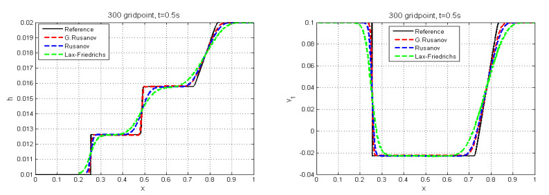
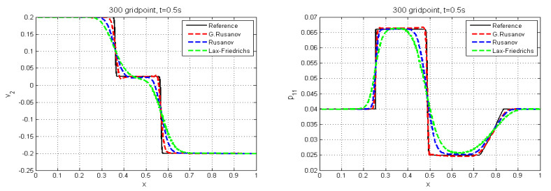
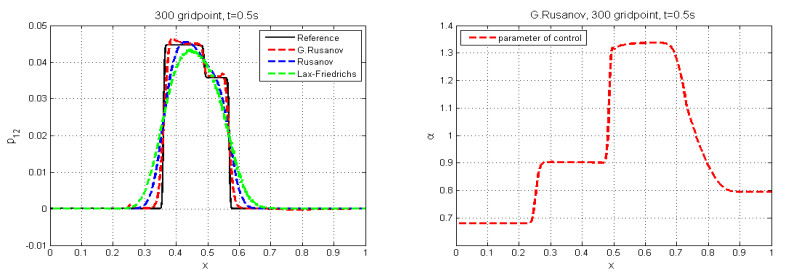
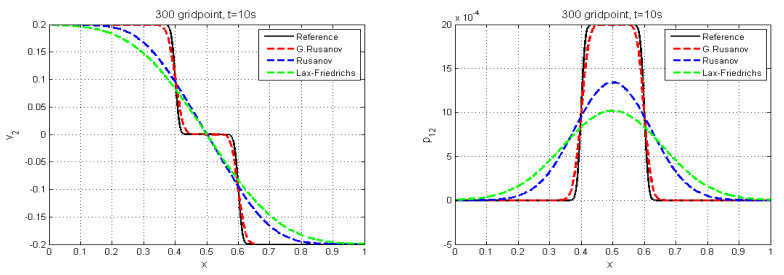
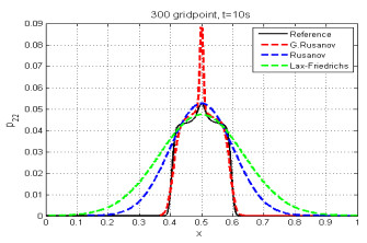
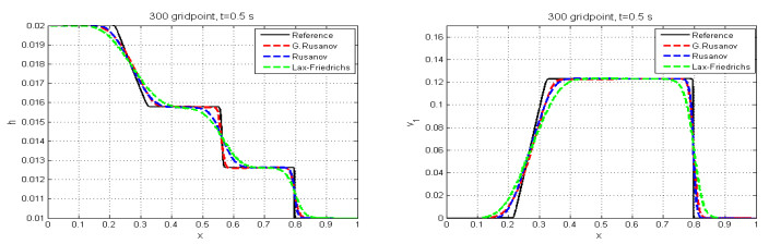
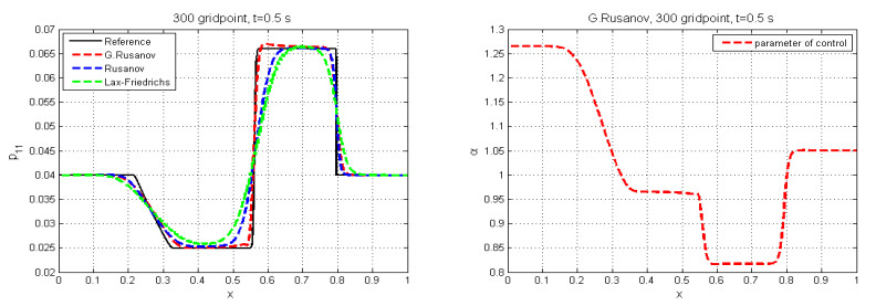
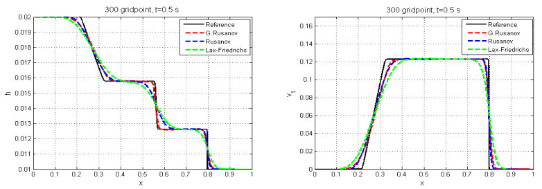
The shear shallow water (SSW) model introduces an approximation for shallow water flows by including the effect of vertical shear in the system. Six non-linear hyperbolic partial differential equations with non-conservative laws make up this system. Shear, contact, rarefaction, and shock waves are all admissible in this model. We developed the finite-volume two-step scheme, the so-called generalized Rusanov (G. Rusanov) scheme, for solving the SSW model. This method is split into two stages. The first one relies on a local parameter that permits control over the diffusion. In stage two, the conservation equation is recovered. Numerous numerical instances were taken into consideration. We clarified that the G. Rusanov scheme satisfied the C-property. We also compared the numerical solutions with those obtained from the Rusanov, Lax-Friedrichs, and reference solutions. Finally, the G. Rusanov technique may be applied for solving a wide range of additional models in developed physics and applied science.

Keywords:

Citation: H. S. Alayachi, Mahmoud A. E. Abdelrahman, Kamel Mohamed. Finite-volume two-step scheme for solving the shear shallow water model[J]. AIMS Mathematics, 2024, 9(8): 20118-20135. doi: 10.3934/math.2024980

Related Papers:

[1]	Ibtisam Aldawish, Mohamed Jleli, Bessem Samet . Blow-up of solutions to fractional differential inequalities involving $\psi$ -Caputo fractional derivatives of different orders. AIMS Mathematics, 2022, 7(5): 9189-9205. doi: 10.3934/math.2022509
[2]	Tao Yan, Ghulam Farid, Sidra Bibi, Kamsing Nonlaopon . On Caputo fractional derivative inequalities by using strongly $(\alpha, h-m)$ -convexity. AIMS Mathematics, 2022, 7(6): 10165-10179. doi: 10.3934/math.2022565
[3]	Muhammad Tariq, Asif Ali Shaikh, Sotiris K. Ntouyas, Jessada Tariboon . Some novel refinements of Hermite-Hadamard and Pachpatte type integral inequalities involving a generalized preinvex function pertaining to Caputo-Fabrizio fractional integral operator. AIMS Mathematics, 2023, 8(11): 25572-25610. doi: 10.3934/math.20231306
[4]	Hadjer Belbali, Maamar Benbachir, Sina Etemad, Choonkil Park, Shahram Rezapour . Existence theory and generalized Mittag-Leffler stability for a nonlinear Caputo-Hadamard FIVP via the Lyapunov method. AIMS Mathematics, 2022, 7(8): 14419-14433. doi: 10.3934/math.2022794
[5]	Choukri Derbazi, Hadda Hammouche . Caputo-Hadamard fractional differential equations with nonlocal fractional integro-differential boundary conditions via topological degree theory. AIMS Mathematics, 2020, 5(3): 2694-2709. doi: 10.3934/math.2020174
[6]	Deepak B. Pachpatte . On some ψ Caputo fractional Čebyšev like inequalities for functions of two and three variables. AIMS Mathematics, 2020, 5(3): 2244-2260. doi: 10.3934/math.2020148
[7]	M. A. Zaky, M. Babatin, M. Hammad, A. Akgül, A. S. Hendy . Efficient spectral collocation method for nonlinear systems of fractional pantograph delay differential equations. AIMS Mathematics, 2024, 9(6): 15246-15262. doi: 10.3934/math.2024740
[8]	M. J. Huntul . Inverse source problems for multi-parameter space-time fractional differential equations with bi-fractional Laplacian operators. AIMS Mathematics, 2024, 9(11): 32734-32756. doi: 10.3934/math.20241566
[9]	Imran Abbas Baloch, Thabet Abdeljawad, Sidra Bibi, Aiman Mukheimer, Ghulam Farid, Absar Ul Haq . Some new Caputo fractional derivative inequalities for exponentially $(\theta, h-m)$ –convex functions. AIMS Mathematics, 2022, 7(2): 3006-3026. doi: 10.3934/math.2022166
[10]	Muhammad Tariq, Hijaz Ahmad, Abdul Ghafoor Shaikh, Soubhagya Kumar Sahoo, Khaled Mohamed Khedher, Tuan Nguyen Gia . New fractional integral inequalities for preinvex functions involving Caputo-Fabrizio operator. AIMS Mathematics, 2022, 7(3): 3440-3455. doi: 10.3934/math.2022191

Abstract

1. Introduction

Time-fractional differential equations arise in the mathematical modeling of a variety of real-world phenomena in many areas of sciences and engineering, such as elasticity, heat transfer, circuits systems, continuum mechanics, fluid mechanics, wave theory, etc. For more details, we refer the reader to ^{[4,6,7,8,14,15,17,24]} and the references therein. Consequently, the study of time-fractional differential equations attracted much attention of many researchers (see e.g. ^{[1,5,9,10,19,22,23]} and the references therein).

Multi-time differential equations arise, for example, in analyzing frequency and amplitude modulation in oscillators, see Narayan and Roychowdhury ^[18]. Some methods for solving Multi-time differential equations can be found in ^[20,21].

The study of blowing-up solutions to time-fractional differential equations was initiated by Kirane and his collaborators, see e.g. ^[3,11,12,13]. In particular, Kirane et al. ^[11] considered the two-times fractional differential equation

$\begin{eqnarray} \left\{\begin{array}{llll} {}^C\!D_{0|t}^\alpha u (t,s)+{}^C\!D_{0|s}^\beta |u|^m (t,s) = |u|^p(t,s),\quad t,s > 0,\\ \\ u(0,s) = u_0(s),\, u(t,0) = u_1(t),\quad t,s > 0, \end{array} \right. \end{eqnarray}$

(1.1)

where $p, m > 1$ , $0 < \alpha, \beta < 1$ , ${}^C\!D_{0|t}^\alpha$ is the Caputo fractional derivative of order $\alpha$ with respect to the first time-variable $t$ , and ${}^C\!D_{0|s}^\beta$ is the Caputo fractional derivative of order $\beta$ with respect to the second time-variable $s$ . Namely, the authors provided sufficient conditions for which any solution to (1.1) blows-up in a finite time. In the same reference, the authors extended their study to the case of systems.

In this paper, we investigate the nonexistence of global solutions to two-times-fractional differential inequalities of the form

$\begin{eqnarray} \left\{\begin{array}{llll} {}^{HC}\!D_{a|t}^\alpha u (t,s)+{}^C\!D_{a|s}^\beta |u|^m (t,s) \geq (s-a)^\gamma \left(\ln \frac{t}{a}\right)^\sigma |u|^p(t,s),\quad t,s > a,\\ \\ u(a,s) = u_0(s),\, u(t,a) = u_1(t),\quad t,s > a, \end{array} \right. \end{eqnarray}$

(1.2)

where $p > 1$ , $m\geq 1$ , $\gamma, \sigma\in \mathbb{R}$ , $a > 0$ , $0 < \alpha, \beta < 1$ , ${}^{HC}\!D_{a|t}^\alpha$ is the Hadamard-Caputo fractional derivative of order $\alpha$ with respect to the first time-variable $t$ , and ${}^C\!D_{a|s}^\beta$ is the Caputo fractional derivative of order $\beta$ with respect to the second time-variable $s$ . Using the test function method (see e.g. ^[16]) and a judicious choice of a test function, we establish sufficient conditions ensuring the nonexistence of global solutions to (1.2). Our obtained conditions depend on the parameters $\alpha, \beta, p, m, \gamma, \sigma$ , and the initial values.

Our motivation for considering problems of type (1.2) is to study the combination effect of the two fractional derivatives of different nature ${}^{HC}\!D_{a|t}^\alpha$ and ${}^C\!D_{a|s}^\beta$ on the nonexistence of global solutions to (1.2). As far as we know, the study of nonexistence of global solutions for time fractional differential equations (or inequalities) involving both Hadamard-Caputo and Caputo fractional derivatives, was never considered in the literature.

The rest of the paper is organized as follows: In Section 2, we recall some concepts from fractional calculus and provide some useful lemmas. In Section 3, we state our main results and provide some examples. Section 4 is devoted to the proofs of our main results.

2. Some preliminaries

Let $a, T\in \mathbb{R}$ be such that $0 < a < T$ . The left-sided and right-sided Riemann-Liouville fractional integrals of order $\theta > 0$ of a function $\vartheta\in L^1([a, T])$ , are defined respectively by (see ^[10])

$(I_a^\theta\vartheta)(t) = \frac{1}{\Gamma(\theta)} \int_a^t (t-\tau)^{\theta-1} \vartheta(\tau)\,d\tau$

and

$(I_T^\theta\vartheta)(t) = \frac{1}{\Gamma(\theta)} \int_t^T (\tau-t)^{\theta-1} \vartheta(\tau)\,d\tau,$

for almost everywhere $t\in [a, T]$ , where $\Gamma$ is the Gamma function.

Notice that, if $\vartheta\in C([a, T])$ , then $I_a^\theta\vartheta, I_T^\theta\vartheta \in C([a, T])$ with

$\begin{equation} (I_a^\theta\vartheta)(a) = (I_T^\theta\vartheta)(T) = 0. \end{equation}$

(2.1)

The Caputo fractional derivative of order $\theta\in (0, 1)$ of a function $\vartheta\in AC([a, \infty))$ , is defined by (see ^[10])

${}^CD_a^\theta \vartheta (t) = (I_a^{1-\theta} \vartheta')(t) = \frac{1}{\Gamma(1-\theta)}\int_a^t (t-\tau)^{-\theta} \vartheta'(\tau)\,d\tau,$

for almost everywhere $t\geq a$ .

Lemma 2.1. [see ^[10]]Let $\kappa > 0$ , $p, q\geq 1$ , and $\frac{1}{p}+\frac{1}{q}\leq 1+\kappa$ ( $p\neq 1$ , $q\neq 1$ , in the case $\frac{1}{p}+\frac{1}{q} = 1+\kappa$ ). Let $\vartheta\in L^p([a, T]$ and $w\in L^q([a, T])$ . Then

$\int_a^T (I_a^\kappa \vartheta)(t) w(t)\,dt = \int_a^T \vartheta(t) (I_T^\kappa w)(t)\,dt.$

The left-sided and right-sided Hadamard fractional integrals of order $\theta > 0$ of a function $\vartheta\in L^1([a, T])$ , are defined respectively by (see ^[10])

$(J_a^\theta\vartheta)(t) = \frac{1}{\Gamma(\theta)} \int_a^t \left(\ln \frac{t}{\tau}\right)^{\theta-1} \vartheta(\tau) \frac{1}{\tau}\,d\tau$

and

$(J_T^\theta\vartheta)(t) = \frac{1}{\Gamma(\theta)} \int_t^T \left(\ln \frac{\tau}{t}\right)^{\theta-1} \vartheta(\tau) \frac{1}{\tau}\,d\tau,$

for almost everywhere $t\in [a, T]$ .

Notice that, if $\vartheta\in C([a, T])$ , then $J_a^\theta\vartheta, J_T^\theta\vartheta \in C([a, T])$ with

$\begin{equation} (J_a^\theta\vartheta)(a) = (J_T^\theta\vartheta)(T) = 0. \end{equation}$

(2.2)

The Hadamard-Caputo fractional derivative of order $\theta\in (0, 1)$ of a function $\vartheta\in AC([a, \infty))$ , is defined by (see ^[2])

${}^{HC}D_a^\theta \vartheta(t) = (J_a^{1-\theta} \delta \vartheta)(t) = \frac{1}{\Gamma(1-\theta)}\int_a^t \left(\ln \frac{t}{\tau}\right)^{-\theta} \delta \vartheta(\tau) \frac{1}{\tau}\,d\tau,$

for almost everywhere $t\geq a$ , where

$\delta \vartheta(t) = t \vartheta'(t).$

We have the following integration by parts rule.

Lemma 2.2. Let $\kappa > 0$ , $p, q\geq 1$ , and $\frac{1}{p}+\frac{1}{q}\leq 1+\kappa$ ( $p\neq 1$ , $q\neq 1$ , in the case $\frac{1}{p}+\frac{1}{q} = 1+\kappa$ ). If $\vartheta \circ \exp \in L^p([\ln a, \ln T])$ and $w \circ \exp \in L^q([\ln a, \ln T])$ , then

$\int_a^T (J_a^\kappa\vartheta)(t) w(t)\frac{1}{t}\,dt = \int_a^T \vartheta(t)(J_T^\kappa w)(t)\frac{1}{t}\,dt.$

Proof. Using the change of variable $x = \ln \tau$ , we obtain

$\begin{eqnarray*} (J_a^\kappa\vartheta)(t)& = &\frac{1}{\Gamma(\kappa)} \int_a^t \left(\ln \frac{t}{\tau}\right)^{\kappa-1} \vartheta(\tau) \frac{1}{\tau}\,d\tau\\ & = & \frac{1}{\Gamma(\kappa)} \int_{\ln a}^{\ln t} \left(\ln t- x\right)^{\kappa-1} (\vartheta\circ \exp) (x)\,dx, \end{eqnarray*}$

that is,

$\begin{equation} (J_a^\kappa\vartheta)(t) = \left(I_{\ln a}^\kappa \vartheta\circ \exp\right) (\ln t). \end{equation}$

(2.3)

Similarly, we have

$\begin{equation} (J_T^\kappa w)(t) = \left(I_{\ln T}^\kappa w\circ \exp\right) (\ln t). \end{equation}$

(2.4)

By (2.3), we obtain

$\int_a^T (J_a^\kappa\vartheta)(t) w(t)\frac{1}{t}\,dt = \int_a^T \left(I_{\ln a}^\kappa \vartheta\circ \exp\right) (\ln t) w(t)\frac{1}{t}\,dt.$

Using the change of variable $x = \ln t$ , we get

$\int_a^T (J_a^\kappa\vartheta)(t) w(t)\frac{1}{t}\,dt = \int_{\ln a}^{\ln T} \left(I_{\ln a}^\kappa \vartheta\circ \exp\right)(x) (w\circ\exp)(x) \,dx.$

Since $\vartheta \circ \exp \in L^p([\ln a, \ln T])$ and $w \circ \exp \in L^q([\ln a, \ln T])$ , by Lemma 2.1, we deduce that

$\int_a^T (J_a^\kappa\vartheta)(t) w(t)\frac{1}{t}\,dt = \int_{\ln a}^{\ln T} (\vartheta\circ \exp)(x) \left(I_{\ln T}^{\kappa} w\circ\exp\right)(x)\,dx.$

Using again the change of variable $x = \ln t$ , there holds

$\int_a^T (J_a^\kappa\vartheta)(t) w(t)\frac{1}{t}\,dt = \int_{a}^{T} \vartheta(t) \left(I_{\ln T}^{\kappa} w\circ\exp\right)(\ln t)\frac{1}{t}\,dt.$

Then, by (2.4), the desired result follows.

By elementary calculations, we obtain the following properties.

Lemma 2.3. For sufficiently large $\lambda$ , let

$\begin{equation} \phi_1(t) = \left(\ln \frac{T}{a}\right)^{-\lambda} \left(\ln \frac{T}{t}\right)^{\lambda},\quad a\leq t\leq T. \end{equation}$

(2.5)

Let $\kappa\in (0, 1)$ . Then

$\begin{eqnarray} (J_{T}^{\kappa}\phi_1)(t)& = & \frac{\Gamma(\lambda+1)}{\Gamma(\kappa+\lambda+1)} \left(\ln \frac{T}{a}\right)^{-\lambda} \left(\ln \frac{T}{t}\right)^{\kappa+\lambda}, \end{eqnarray}$

(2.6)

$\begin{eqnarray} (J_{T}^{\kappa}\phi_1)'(t)& = &-\frac{\Gamma(\lambda+1)}{\Gamma(\kappa+\lambda)} \left(\ln \frac{T}{a}\right)^{-\lambda} \left(\ln \frac{T}{t}\right)^{\kappa+\lambda-1} \frac{1}{t}. \end{eqnarray}$

(2.7)

Lemma 2.4. For sufficiently large $\lambda$ , let

$\begin{equation} \phi_2(s) = (T-a)^{-\lambda} (T-s)^{\lambda},\quad a\leq s\leq T. \end{equation}$

(2.8)

Let $\kappa\in (0, 1)$ . Then

$\begin{eqnarray} (I_{T}^{\kappa}\phi_2)(s)& = & \frac{\Gamma(\lambda+1)}{\Gamma(\kappa+\lambda+1)} (T-a)^{-\lambda} (T-s)^{\kappa+\lambda}, \end{eqnarray}$

(2.9)

$\begin{eqnarray} (I_{T}^{\kappa}\phi_2)'(s)& = &-\frac{\Gamma(\lambda+1)}{\Gamma(\kappa+\lambda)} (T-a)^{-\lambda} (T-s)^{\kappa+\lambda-1}. \end{eqnarray}$

(2.10)

3. Main results

First, let us define global solutions to (1.2). To do this, we need to introduce the functional space

$X_a: = \left\{u\in C([a,\infty)\times [a,\infty)):\, u(\cdot,s)\in AC([a,\infty)),\, |u|^m(t,\cdot)\in AC([a,\infty))\right\}.$

We say that $u$ is a global solution to (1.2), if $u\in X_a$ and $u$ satisfies the fractional differential inequality

${}^{HC}\!D_{a|t}^\alpha u (t,s)+{}^C\!D_{a|s}^\beta |u|^m (t,s) \geq (s-a)^\gamma \left(\ln \frac{t}{a}\right)^\sigma |u|^p(t,s)$

for almost everywhere $t, s\geq a$ , as well as the initial conditions

$u(a,s) = u_0(s),\, u(t,a) = u_1(t),\quad t,s > a.$

Now, we state our main results.

Theorem 3.1. Let $u_0\in L^1([a, \infty))$ , $u_1\in L^m([a, \infty), \frac{1}{t}\, dt)$ , and $u_1\not\equiv 0$ .Let

$\begin{equation} 0 < \beta < \frac{1}{m}\leq 1,\quad \gamma > \max\left\{\frac{m-1}{1-m\beta}, m(\sigma+1)-1\right\}\beta. \end{equation}$

(3.1)

$\begin{equation} m\max\left\{\gamma+1,\sigma+1\right\} < p < 1+\frac{\gamma}{\beta}, \end{equation}$

(3.2)

then, for all $\alpha\in (0, 1)$ , (1.2) admits no global solution.

Remark 3.1. Notice that by (3.1), the set of exponents $p$ satisfying (3.2) is nonempty.

Theorem 3.2. Let $u_0\in L^1([a, \infty))$ , $u_1\in L^m([a, \infty), \frac{1}{t}\, dt)$ , and $u_1\not\equiv 0$ . Let

$\begin{equation} 0 < \beta < \frac{1}{m}\leq 1,\quad 1-\frac{1}{m} < \alpha < 1,\quad \sigma > \frac{(m-1)(1-\alpha)}{1-m\beta}-\alpha. \end{equation}$

(3.3)

$\begin{equation} \beta \max\left\{ \frac{m-1}{1-m\beta},m(\sigma+1)-1\right\} < \gamma < \frac{(\sigma+\alpha)\beta}{1-\alpha} \end{equation}$

(3.4)

and

$\begin{equation} p = 1+\frac{\gamma}{\beta}, \end{equation}$

(3.5)

then (1.2) admits no global solution.

Remark 3.2. Notice that by (3.3), the set of real numbers $\gamma$ satisfying (3.4) is nonempty.

We illustrate our obtained results by the following examples.

Example 3.1. Consider the fractional differential inequality

$\begin{eqnarray} \left\{\begin{array}{llll} {}^{HC}\!D_{a|t}^\alpha u (t,s)+{}^C\!D_{a|s}^{\frac{1}{4}} u^2 (t,s) \geq (s-a) \left(\ln \frac{t}{a}\right)^{-1} |u|^p(t,s),\quad t,s > a,\\ \\ u(a,s) = (1+s^2)^{-1},\, u(t,a) = \exp(-t),\quad t,s > a, \end{array} \right. \end{eqnarray}$

(3.6)

where $a > 0$ and $0 < \alpha < 1$ . Observe that (3.6) is a special case of (1.2) with

$\beta = \frac{1}{4},\,\, m = 2,\,\, \sigma = -1,\,\,\gamma = 1,\,\, u_0(s) = (1+s^2)^{-1},\,\, u_1(t) = \exp(-t).$

Moreover, we have

$0 < \beta = \frac{1}{4} < \frac{1}{2} = \frac{1}{m} < 1, \quad \max\left\{\frac{m-1}{1-m\beta}, m(\sigma+1)-1\right\}\beta = \frac{\max\{2,0\}}{4} = \frac{1}{2} < \gamma = 1,$

and $u_0\in L^1([a, \infty))$ , $u_1\in L^m([a, \infty), \frac{1}{t}\, dt)$ . Hence, condition (3.1) is satisfied. Then, by Theorem 3.1, we deduce that, if

$m\max\left\{\gamma+1,\sigma+1\right\} < p < 1+\frac{\gamma}{\beta},$

that is,

$4 < p < 5,$

then (3.6) admits no global solution.

Example 3.2. Consider the fractional differential inequality

$\begin{eqnarray} \left\{\begin{array}{llll} {}^{HC}\!D_{a|t}^{\frac{3}{4}} u (t,s)+{}^C\!D_{a|s}^{\frac{1}{2}} |u| (t,s) \geq (s-a)^{\frac{1}{4}} \left(\ln \frac{t}{a}\right)^{-\frac{1}{2}} |u|^{\frac{3}{2}}(t,s),\quad t,s > a,\\ \\ u(a,s) = (1+s^2)^{-1},\, u(t,a) = \exp(-t),\quad t,s > a, \end{array} \right. \end{eqnarray}$

(3.7)

where $a > 0$ . Then (3.7) is a special case of (1.2) with

$\alpha = \frac{3}{4},\,\, \beta = \frac{1}{2},\,\, m = 1,\,\, \sigma = -\frac{1}{2},\,\, \gamma = \frac{1}{4},\,\, p = \frac{3}{2},\,\, u_0(s) = (1+s^2)^{-1},\,\, u_1(t) = \exp(-t).$

On the other hand, we have

$0 < \beta = \frac{1}{2} < 1 = \frac{1}{m},\quad 1-\frac{1}{m} = 0 < \alpha = \frac{3}{4} < 1,\quad \sigma = -\frac{1}{2} > -\frac{3}{4} = \frac{(m-1)(1-\alpha)}{1-m\beta}-\alpha,$

which shows that condition (3.3) is satisfied. Moreover, we have

$\beta \max\left\{\frac{m-1}{1-m\beta},m(\sigma+1)-1\right\} = -\frac{1}{4} < \gamma = \frac{1}{4} < \frac{1}{2} = \frac{(\sigma+\alpha)\beta}{1-\alpha},\quad p = \frac{3}{2} = 1+\frac{\gamma}{\beta},$

which shows that conditions (3.4) and (3.5) are satisfied. Then, by Theorem 3.2, we deduce that (3.7) admits no global solution.

4. Proofs of the main results

In this section, $C$ denotes a positive constant independent on $T$ , whose value may change from line to line.

Proof of Theorem 3.1. Suppose that $u\in X_a$ is a global solution to (1.2). For sufficiently large $T$ and $\lambda$ , let

$\varphi(t,s) = \phi_1(t)\phi_2(s),\quad a\leq t,s\leq T,$

where $\phi_1$ and $\phi_2$ are defined respectively by (2.5) and (2.8). Multiplying the inequality in (1.2) by $\frac{1}{t}\varphi$ and integrating over $\Omega_T: = (a, T)\times (a, T)$ , we obtain

$\begin{equation} \begin{aligned} &\int_{\Omega_T} (s-a)^\gamma \left(\ln \frac{t}{a}\right)^\sigma |u|^p \varphi(t,s)\frac{1}{t}\,dt\,ds\\ & \leq \int_{\Omega_T}{}^{HC}\!D_{a|t}^\alpha u \,\varphi(t,s)\frac{1}{t}\,dt\,ds + \int_{\Omega_T} {}^C\!D_{a|s}^\beta |u|^m\,\varphi(t,s)\frac{1}{t}\,dt\,ds. \end{aligned} \end{equation}$

(4.1)

On the other hand, using Lemma 2.2, integrating by parts, using the initial conditions, and taking in consideration (2.2), we obtain

$\begin{aligned} &\int_a^T {}^{HC}\!D_{a|t}^\alpha u \,\varphi(t,s)\frac{1}{t}\,dt\\ & = \int_a^T \left(J_{a|t}^{1-\alpha} t \frac{\partial u}{\partial t}\right)(t,s)\varphi(t,s)\frac{1}{t}\,dt\\ & = \int_a^T \frac{\partial u}{\partial t}(t,s) \left(J_{T|t}^{1-\alpha}\varphi\right)(t,s) \,dt\\ & = \left[u(t,s) \left(J_{T|t}^{1-\alpha}\varphi\right)(t,s)\right]_{t = a}^T-\int_a^T u(t,s) \frac{\partial \left(J_{T|t}^{1-\alpha}\varphi\right)}{\partial t}(t,s)\,dt\\ & = -u_0(s)\left(J_{T|t}^{1-\alpha}\varphi\right)(a,s)-\int_a^T u(t,s) \frac{\partial \left(J_{T|t}^{1-\alpha}\varphi\right)}{\partial t}(t,s)\,dt. \end{aligned}$

Integrating over $(a, T)$ , we get

$\begin{equation} \begin{aligned} &\int_{\Omega_T}{}^{HC}\!D_{a|t}^\alpha u \,\varphi(t,s)\frac{1}{t}\,dt\,ds\\ & = -\int_a^T u_0(s)\left(J_{T|t}^{1-\alpha}\varphi\right)(a,s)\,ds-\int_{\Omega_T} u(t,s) \frac{\partial \left(J_{T|t}^{1-\alpha}\varphi\right)}{\partial t}(t,s)\,dt\,ds. \end{aligned} \end{equation}$

(4.2)

Similarly, using Lemma 2.1, integrating by parts, using the initial conditions, and taking in consideration (2.1), we obtain

$\begin{aligned} & \int_a^T {}^C\!D_{a|s}^\beta |u|^m\,\varphi(t,s)\,ds\\ & = \int_a^T \left(I_{a|s}^{1-\beta} \frac{\partial |u|^m}{\partial s}(t,s)\right)\,\varphi(t,s)\,ds\\ & = \int_a^T \frac{\partial |u|^m}{\partial s}(t,s) \left(I_{T|s}^{1-\beta}\varphi\right)(t,s)\,ds\\ & = \left[|u|^m(t,s)\left(I_{T|s}^{1-\beta}\varphi\right)(t,s)\right]_{s = a}^T-\int_a^T |u|^m(t,s) \frac{\partial \left(I_{T|s}^{1-\beta}\varphi\right)}{\partial s}(t,s)\,ds\\ & = -|u_1(t)|^m \left(I_{T|s}^{1-\beta}\varphi\right)(t,a)-\int_a^T |u|^m(t,s) \frac{\partial \left(I_{T|s}^{1-\beta}\varphi\right)}{\partial s}(t,s)\,ds. \end{aligned}$

Integrating over $(a, T)$ , there holds

$\begin{equation} \begin{aligned} &\int_{\Omega_T} {}^C\!D_{a|s}^\beta |u|^m\,\varphi(t,s)\frac{1}{t}\,dt\,ds\\ & = -\int_a^T |u_1(t)|^m \left(I_{T|s}^{1-\beta}\varphi\right)(t,a)\frac{1}{t}\,dt-\int_{\Omega_T}|u|^m(t,s) \frac{\partial \left(I_{T|s}^{1-\beta}\varphi\right)}{\partial s}(t,s)\frac{1}{t}\,dt\,\,ds. \end{aligned} \end{equation}$

(4.3)

It follows from (4.1)–(4.3) that

$\begin{equation} \begin{aligned} &\int_{\Omega_T} (s-a)^\gamma \left(\ln \frac{t}{a}\right)^\sigma |u|^p \varphi(t,s)\frac{1}{t}\,dt\,ds\\ &+\int_a^T u_0(s)\left(J_{T|t}^{1-\alpha}\varphi\right)(a,s)\,ds +\int_a^T |u_1(t)|^m \left(I_{T|s}^{1-\beta}\varphi\right)(t,a)\frac{1}{t}\,dt\\ &\leq \int_{\Omega_T} |u| \left|\frac{\partial \left(J_{T|t}^{1-\alpha}\varphi\right)}{\partial t}\right|\,dt\,ds+\int_{\Omega_T}|u|^m \left|\frac{\partial \left(I_{T|s}^{1-\beta}\varphi\right)}{\partial s}\right|\frac{1}{t}\,dt\,\,ds. \end{aligned} \end{equation}$

(4.4)

On the other hand, by Young's inequality, we have

$\begin{equation} \begin{aligned} &\int_{\Omega_T} |u| \left|\frac{\partial \left(J_{T|t}^{1-\alpha}\varphi\right)}{\partial t}\right|\,dt\,ds\\ &\leq \frac{1}{2} \int_{\Omega_T} (s-a)^\gamma \left(\ln \frac{t}{a}\right)^\sigma |u|^p \varphi(t,s)\frac{1}{t}\,dt\,ds\\ &+C \int_{\Omega_T} t^{\frac{1}{p-1}} (s-a)^{\frac{-\gamma}{p-1}} \left(\ln \frac{t}{a}\right)^{\frac{-\sigma}{p-1}} \varphi^{\frac{-1}{p-1}}(t,s) \left|\frac{\partial \left(J_{T|t}^{1-\alpha}\varphi\right)}{\partial t}\right|^{\frac{p}{p-1}}\,dt\,ds. \end{aligned} \end{equation}$

(4.5)

Similarly, since $p > m$ , we have

$\begin{equation} \begin{aligned} &\int_{\Omega_T}|u|^m \left|\frac{\partial \left(I_{T|s}^{1-\beta}\varphi\right)}{\partial s}\right|\frac{1}{t}\,dt\,\,ds\\ &\leq \frac{1}{2} \int_{\Omega_T} (s-a)^\gamma \left(\ln \frac{t}{a}\right)^\sigma |u|^p \varphi(t,s)\frac{1}{t}\,dt\,ds\\ &+C \int_{\Omega_T} \frac{1}{t} (s-a)^{\frac{-\gamma m}{p-m}} \left(\ln \frac{t}{a}\right)^{\frac{-\sigma m}{p-m}} \varphi^{\frac{-m}{p-m}}(t,s) \left|\frac{\partial \left(I_{T|s}^{1-\beta}\varphi\right)}{\partial s}\right|^{\frac{p}{p-m}}\,dt\,\,ds. \end{aligned} \end{equation}$

(4.6)

Hence, combining (4.4)–(4.6), we deduce that

$\begin{equation} \int_a^T u_0(s)\left(J_{T|t}^{1-\alpha}\varphi\right)(a,s)\,ds +\int_a^T |u_1(t)|^m \left(I_{T|s}^{1-\beta}\varphi\right)(t,a)\frac{1}{t}\,dt\leq C (K_1+K_2), \end{equation}$

(4.7)

where

$K_1 = \int_{\Omega_T} t^{\frac{1}{p-1}} (s-a)^{\frac{-\gamma}{p-1}} \left(\ln \frac{t}{a}\right)^{\frac{-\sigma}{p-1}} \varphi^{\frac{-1}{p-1}}(t,s) \left|\frac{\partial \left(J_{T|t}^{1-\alpha}\varphi\right)}{\partial t}\right|^{\frac{p}{p-1}}\,dt\,ds$

and

$K_2 = \int_{\Omega_T} \frac{1}{t} (s-a)^{\frac{-\gamma m}{p-m}} \left(\ln \frac{t}{a}\right)^{\frac{-\sigma m}{p-m}} \varphi^{\frac{-m}{p-m}}(t,s) \left|\frac{\partial \left(I_{T|s}^{1-\beta}\varphi\right)}{\partial s}\right|^{\frac{p}{p-m}}\,dt\,\,ds.$

By the definition of the function $\varphi$ , we have

$\left(J_{T|t}^{1-\alpha}\varphi\right)(a,s) = \phi_2(s) \left(J_{T|t}^{1-\alpha}\phi_1\right)(a).$

Thus, using (2.6), we obtain

$\left(J_{T|t}^{1-\alpha}\varphi\right)(a,s) = C \phi_2(s) \left(\ln \frac{T}{a}\right)^{1-\alpha}.$

Integrating over $(a, T)$ , we get

$\begin{equation} \int_a^T u_0(s)\left(J_{T|t}^{1-\alpha}\varphi\right)(a,s)\,ds = C \left(\ln \frac{T}{a}\right)^{1-\alpha} \int_a^T u_0(s)(T-a)^{-\lambda} (T-s)^{\lambda}\,ds. \end{equation}$

(4.8)

Similarly, by the definition of the function $\varphi$ , we have

$\left(I_{T|s}^{1-\beta}\varphi\right)(t,a) = \phi_1(t) \left(I_{T|s}^{1-\beta}\phi_2\right)(a).$

Thus, using (2.9), we obtain

$\left(I_{T|s}^{1-\beta}\varphi\right)(t,a) = C \phi_1(t)(T-a)^{1-\beta}.$

Integrating over $(a, T)$ , we get

$\begin{equation} \int_a^T |u_1(t)|^m \left(I_{T|s}^{1-\beta}\varphi\right)(t,a)\frac{1}{t}\,dt = C (T-a)^{1-\beta} \int_a^T |u_1(t)|^m \left(\ln \frac{T}{a}\right)^{-\lambda} \left(\ln \frac{T}{t}\right)^{\lambda}\frac{1}{t}\,dt. \end{equation}$

(4.9)

Combining (4.8) with (4.9), there holds

$\begin{aligned} &\int_a^T u_0(s)\left(J_{T|t}^{1-\alpha}\varphi\right)(a,s)\,ds+ \int_a^T |u_1(t)|^m \left(I_{T|s}^{1-\beta}\varphi\right)(t,a)\frac{1}{t}\,dt\\ & = C \left(\ln \frac{T}{a}\right)^{1-\alpha} \int_a^T u_0(s)(T-a)^{-\lambda} (T-s)^{\lambda}\,ds\\ &+C (T-a)^{1-\beta} \int_a^T |u_1(t)|^m \left(\ln \frac{T}{a}\right)^{-\lambda} \left(\ln \frac{T}{t}\right)^{\lambda}\frac{1}{t}\,dt. \end{aligned}$

Since $u_0\in L^1([a, \infty))$ , $u_1\in L^m([a, \infty), \frac{1}{t}\, dt)$ , and $u_1\not\equiv 0$ , by the dominated convergence theorem, we deduce that for sufficiently large $T$ ,

$\begin{equation} \begin{aligned} &\int_a^T u_0(s)\left(J_{T|t}^{1-\alpha}\varphi\right)(a,s)\,ds+ \int_a^T |u_1(t)|^m \left(I_{T|s}^{1-\beta}\varphi\right)(t,a)\frac{1}{t}\,dt\\ &\geq C (T-a)^{1-\beta} \int_a^\infty |u_1(t)|^m \frac{1}{t}\,dt. \end{aligned} \end{equation}$

(4.10)

Now, we shall estimate the terms $K_i$ , $i = 1, 2$ . By the definition of the function $\varphi$ , the term $K_1$ can be written as

$\begin{equation} K_1 = \left(\int_a^T (s-a)^{\frac{-\gamma}{p-1}} \phi_2(s)\,ds\right) \left(\int_a^T t^{\frac{1}{p-1}} \left(\ln \frac{t}{a}\right)^{\frac{-\sigma}{p-1}} \phi_1^{\frac{-1}{p-1}}(t) \left|\left(J_{T|t}^{1-\alpha}\phi_1\right)'(t)\right|^{\frac{p}{p-1}}\,dt\right). \end{equation}$

(4.11)

Next, by (2.8), we obtain

$\begin{eqnarray*} \int_a^T (s-a)^{\frac{-\gamma}{p-1}} \phi_2(s)\,ds& = & (T-a)^{-\lambda} \int_a^T (s-a)^{\frac{-\gamma}{p-1}} (T-s)^\lambda\,ds\\ &\leq & \int_a^T (s-a)^{\frac{-\gamma}{p-1}}\,ds. \end{eqnarray*}$

On the other hand, by (3.1) and (3.2), it is clear that $\gamma < p-1$ . Thus, we deduce that

$\begin{equation} \int_a^T (s-a)^{\frac{-\gamma}{p-1}} \phi_2(s)\,ds\leq C (T-a)^{1-\frac{\gamma}{p-1}}. \end{equation}$

(4.12)

By (2.5) and (2.7), we have

$\begin{aligned} & \int_a^T t^{\frac{1}{p-1}} \left(\ln \frac{t}{a}\right)^{\frac{-\sigma}{p-1}} \phi_1^{\frac{-1}{p-1}}(t) \left|\left(J_{T|t}^{1-\alpha}\phi_1\right)'(t)\right|^{\frac{p}{p-1}}\,dt\\ & = \left(\ln \frac{T}{a}\right)^{-\lambda} \int_a^T \left(\ln \frac{T}{t}\right)^{\lambda-\frac{\alpha p}{p-1}} \left(\ln \frac{t}{a}\right)^{\frac{-\sigma}{p-1}} \frac{1}{t}\,dt\\ &\leq \left(\ln \frac{T}{a}\right)^{-\frac{\alpha p}{p-1}} \int_a^T \left(\ln \frac{t}{a}\right)^{\frac{-\sigma}{p-1}} \frac{1}{t}\,dt. \end{aligned}$

Notice that by (3.1) and (3.2), we have $\sigma < p-1$ . Thus, we get

$\begin{equation} \begin{aligned} & \int_a^T t^{\frac{1}{p-1}} \left(\ln \frac{t}{a}\right)^{\frac{-\sigma}{p-1}} \phi_1^{\frac{-1}{p-1}}(t) \left|\left(J_{T|t}^{1-\alpha}\phi_1\right)'(t)\right|^{\frac{p}{p-1}}\,dt\\ &\leq C \left(\ln \frac{T}{a}\right)^{1-\frac{\alpha p+\sigma}{p-1}}. \end{aligned} \end{equation}$

(4.13)

Hence, it follows from (4.11)–(4.13) that

$\begin{equation} K_1\leq C (T-a)^{1-\frac{\gamma}{p-1}} \left(\ln \frac{T}{a}\right)^{1-\frac{\alpha p+\sigma}{p-1}}. \end{equation}$

(4.14)

Similarly, we can write the term $K_2$ as

$\begin{equation} K_2 = \left(\int_a^T \frac{1}{t} \left(\ln \frac{t}{a}\right)^{\frac{-\sigma m}{p-m}}\phi_1(t)\,dt\right) \left(\int_a^T (s-a)^{\frac{-\gamma m}{p-m}} \phi_2^{\frac{-m}{p-m}}(s) \left|\left(I_{T|s}^{1-\beta}\phi_2\right)'(s)\right|^{\frac{p}{p-m}}\,ds\right). \end{equation}$

(4.15)

By (2.5), we have

$\begin{eqnarray*} \int_a^T \frac{1}{t} \left(\ln \frac{t}{a}\right)^{\frac{-\sigma m}{p-m}}\phi_1(t)\,dt& = & \left(\ln \frac{T}{a}\right)^{-\lambda} \int_a^T \left(\ln \frac{t}{a}\right)^{\frac{-\sigma m}{p-m}} \left(\ln \frac{T}{t}\right)^{\lambda} \frac{1}{t}\,dt\\ &\leq & \int_a^T \left(\ln \frac{t}{a}\right)^{\frac{-\sigma m}{p-m}}\frac{1}{t}\,dt. \end{eqnarray*}$

Notice that by (3.2), we have $\sigma m < p-m$ . Thus, we get

$\begin{equation} \int_a^T \frac{1}{t} \left(\ln \frac{t}{a}\right)^{\frac{-\sigma m}{p-m}}\phi_1(t)\,dt\leq C \left(\ln \frac{T}{a}\right)^{1-\frac{\sigma m}{p-m}}. \end{equation}$

(4.16)

On the other hand, by (2.8) and (2.10), we have

$\begin{aligned} &\int_a^T (s-a)^{\frac{-\gamma m}{p-m}} \phi_2^{\frac{-m}{p-m}}(s) \left|\left(I_{T|s}^{1-\beta}\phi_2\right)'(s)\right|^{\frac{p}{p-m}}\,ds\\ & = (T-a)^{-\lambda} \int_a^T (T-s)^{\lambda-\frac{\beta p}{p-m}} (s-a)^{\frac{-\gamma m}{p-m}}\,ds \\ &\leq (T-a)^{-\frac{\beta p}{p-m}} \int_a^T(s-a)^{\frac{-\gamma m}{p-m}}\,ds. \end{aligned}$

Notice that by (3.2), we have $p > m(\gamma+1)$ . Therefore, we obtain

$\begin{equation} \int_a^T (s-a)^{\frac{-\gamma m}{p-m}} \phi_2^{\frac{-m}{p-m}}(s) \left|\left(I_{T|s}^{1-\beta}\phi_2\right)'(s)\right|^{\frac{p}{p-m}}\,ds\leq C (T-a)^{1- \frac{\gamma m+\beta p}{p-m}}. \end{equation}$

(4.17)

Combining (4.16) with (4.17), there holds

$\begin{equation} K_2\leq C \left(\ln \frac{T}{a}\right)^{1-\frac{\sigma m}{p-m}}(T-a)^{1- \frac{\gamma m+\beta p}{p-m}}. \end{equation}$

(4.18)

Hence, it follows from (4.14) and (4.18) that

$\begin{equation} K_1+K_2\leq C\left[\left(\ln \frac{T}{a}\right)^{1-\frac{\alpha p+\sigma}{p-1}}(T-a)^{1-\frac{\gamma}{p-1}} +\left(\ln \frac{T}{a}\right)^{1-\frac{\sigma m}{p-m}}(T-a)^{1- \frac{\gamma m+\beta p}{p-m}}\right]. \end{equation}$

(4.19)

Thus, by (4.7), (4.10), and (4.19), we deduce that

$\begin{equation} \begin{aligned} &\int_a^\infty |u_1(t)|^m \frac{1}{t}\,dt\\ &\leq C\left[\left(\ln \frac{T}{a}\right)^{1-\frac{\alpha p+\sigma}{p-1}}(T-a)^{\beta-\frac{\gamma}{p-1}} +\left(\ln \frac{T}{a}\right)^{1-\frac{\sigma m}{p-m}}(T-a)^{\beta- \frac{\gamma m+\beta p}{p-m}}\right]. \end{aligned} \end{equation}$

(4.20)

Notice that by (3.1) and (3.2), we have

$\beta-\frac{\gamma}{p-1} < 0,\quad \beta- \frac{\gamma m+\beta p}{p-m} < 0.$

Hence, passing to the limit as $T\to \infty$ in (4.20), we obtain a contradiction with $u_1\not\equiv 0$ . Consequently, (1.2) admits no global solution. The proof is completed.

Proof of Theorem 3.2. Suppose that $u\in X_a$ is a global solution to (1.2). Notice that in the proof of Theorem 3.1, to obtain (4.20), we used that

$p > m\geq 1,\quad p > \sigma+1,\quad p > m(\sigma+1),\quad p > m(\gamma+1).$

On the other hand, by (3.3)–(3.5), it can be easily seen that the above conditions are satisfied. Thus, (4.20) holds. Hence, taking $p = 1+\frac{\gamma}{\beta}$ in (4.20), we obtain

$\begin{equation} \int_a^\infty |u_1(t)|^m \frac{1}{t}\,dt \leq C\left[\left(\ln \frac{T}{a}\right)^{1-\frac{\alpha p+\sigma}{p-1}}+\left(\ln \frac{T}{a}\right)^{1-\frac{\sigma m}{p-m}}(T-a)^{\beta- \frac{\gamma m+\beta p}{p-m}}\right]. \end{equation}$

(4.21)

On the other hand, by (3.3)–(3.5), we have

$1-\frac{\alpha p+\sigma}{p-1} < 0,\quad \beta- \frac{\gamma m+\beta p}{p-m} < 0.$

Hence, passing to the limit as $T\to \infty$ in (4.21), we obtain a contradiction with $u_1\not\equiv 0$ . This shows that (1.2) admits no global solution. The proof is completed.

5. Conclusions

The two-times fractional differential inequality (1.2) is investigated. Namely, using the test function method and a judicious choice of a test function, sufficient conditions ensuring the nonexistence of global solutions to (1.2) are obtained. Two cases are discussed separately: $1 < p < 1+\frac{\gamma}{\beta}$ (see Theorem 3.1) and $p = 1+\frac{\gamma}{\beta}$ (see Theorem 3.2). In the first case, no assumption is imposed on the fractional order $\alpha\in (0, 1)$ of the Hadamard-Caputo fractional derivative, while in the second case, it is supposed that $\alpha > 1-\frac{1}{m}$ . About the initial conditions, in both cases, it is assumed that $u_0\in L^1([a, \infty))$ , $u_1\in L^m([a, \infty), \frac{1}{t}\, dt)$ , and $u_1\not\equiv 0$ .

Finally, it would be interesting to extend this study to two-times fractional evolution equations. For instance, the tow-times fractional semi-linear heat equation

$\begin{eqnarray*} \left\{\begin{array}{llll} {}^{HC}\!D_{a|t}^\alpha u (t,s,x)+{}^C\!D_{a|s}^\beta |u|^m (t,s,x) \geq (s-a)^\gamma \left(\ln \frac{t}{a}\right)^\sigma |u|^p(t,s,x),\quad t,s > a,\, x\in \mathbb{R}^N,\\ \\ u(a,s,x) = u_0(s,x),\, u(t,a,x) = u_1(t,x),\quad t,s > a, \, x\in \mathbb{R}^N, \end{array} \right. \end{eqnarray*}$

deserves to be studied.

Acknowledgments

The authors extend their appreciation to the Deanship of Scientific Research at Imam Mohammad Ibn Saud Islamic University for funding this work through Research Group no. RG-21-09-02.

Conflict of interest

The authors declare that they have no competing interests.

References

[1]	G. B. Whitham, Linear and nonlinear waves, Hoboken: John Wiley & Sons, 1999. http://doi.org/10.1002/9781118032954
[2]	M. A. E. Abdelrahman, On the shallow water equations, ZNA, 72 (2017), 873–879. https://doi.org/10.1515/zna-2017-0146 doi: 10.1515/zna-2017-0146
[3]	K. Mohamed, S. Sahmim, F. Benkhaldoun, M. A. E. Abdelrahman, Some recent finite volume schemes for one and two layers shallow water equations with variable density, Math. Methods Appl. Sci., 46 (2023), 12979–12995. https://doi.org/10.1002/mma.9227 doi: 10.1002/mma.9227
[4]	K. Mohamed, H. S. Alayachi, M. A. E. Abdelrahman, The mR scheme to the shallow water equation with horizontal density gradients in one and two dimensions, AIMS Mathematics, 8 (2023), 25754–25771. http://doi.org/10.3934/math.20231314 doi: 10.3934/math.20231314
[5]	J. Ren, O. A. Ilhan, H. Bulut, J. Manafian, Multiple rogue wave, dark, bright, and solitary wave solutions to the KP–BBM equation, J. Geom. Phys., 164 (2021), 104159. https://doi.org/10.1016/j.geomphys.2021.104159 doi: 10.1016/j.geomphys.2021.104159
[6]	X. Zhou, O. A. Ilhan, J. Manafian, G. Singh, N. S. Tuguz, N-lump and interaction solutions of localized waves to the (2+1)-dimensional generalized KDKK equation, J. Geom. Phys., 168 (2021), 104312. https://doi.org/10.1016/j.geomphys.2021.104312 doi: 10.1016/j.geomphys.2021.104312
[7]	X. Hong, J. Manafian, O. A. Ilhan, A. I. A. Alkireet, M. K. M. Nasution, Multiple soliton solutions of the generalized Hirota-Satsuma-Ito equation arising in shallow water wave, J. Geom. Phys., 170 (2021), 104338. https://doi.org/10.1016/j.geomphys.2021.104338 doi: 10.1016/j.geomphys.2021.104338
[8]	W. Cai, R. Mohammaditab, G. Fathi, K. Wakil, A. G. Ebadi, N. Ghadimi, Optimal bidding and offering strategies of compressed air energy storage: A hybrid robust-stochastic approach, Renewable Energy, 143 (2019), 1–8. https://doi.org/10.1016/j.renene.2019.05.008 doi: 10.1016/j.renene.2019.05.008
[9]	V. M. Teshukov, Gas-dynamic analogy for vortex free-boundary flows, J. Appl. Mech. Tech. Phys., 48 (2007), 303–309. https://doi.org/10.1007/s10808-007-0039-2 doi: 10.1007/s10808-007-0039-2
[10]	M. M. A. Khater, S. H. Alfalqi, J. F. Alzaidi, S. A. Salama, F. Wang, Plenty of wave solutions to the ill-posed Boussinesq dynamic wave equation under shallow water beneath gravity, AIMS Mathematics, 7 (2022), 54–81. http://doi.org/10.3934/math.2022004 doi: 10.3934/math.2022004
[11]	A. I. Delis, H. Guillard, Y. C. Tai, Numerical simulations of hydraulic jumps with the shear shallow water model, SMAI J. Comput. Math., 4 (2018), 319–344. http://doi.org/10.5802/smai-jcm.37 doi: 10.5802/smai-jcm.37
[12]	J. Zhang, F. Wang, S. Nadeem, M. Sun, Simulation of linear and nonlinear advection-diffusion problems by the direct radial basis function collocation method, Int. Commun. Heat Mass Trans., 130 (2022), 105775. https://doi.org/10.1016/j.icheatmasstransfer.2021.105775 doi: 10.1016/j.icheatmasstransfer.2021.105775
[13]	F. Wang, E. Hou, I. Ahmad, H. Ahmad, Y. Gu, An efficient meshless method for hyperbolic telegraph equations in (1+1) dimensions, Comput. Model. Eng. Sci., 128 (2021), 687–698. https://doi.10.32604/cmes.2021.014739 doi: 10.32604/cmes.2021.014739
[14]	Z. Zhang, F. Wang, J. Zhang, The space-time meshless methods for the solution of one-dimensional Klein-Gordon equations, Wuhan Univ. J. Nat. Sci., 27 (2022), 313–320. https://doi.10.1051/wujns/2022274313 doi: 10.1051/wujns/2022274313
[15]	O. A. Ilhan, J. Manafian, M. Shahriari, Lump wave solutions and the interaction phenomenon for a variable-coefficient Kadomtsev–Petviashvili equation, Comput. Math. Appl., 78 (2019), 2429–2448. https://doi.org/10.1016/j.camwa.2019.03.048 doi: 10.1016/j.camwa.2019.03.048
[16]	H. Zhang, J. Manafian, G. Singh, O. A. Ilhan, A. O. Zekiy, N-lump and interaction solutions of localized waves to the (2+1)-dimensional generalized KP equation, Results Phys., 25 (2021), 104168. https://doi.org/10.1016/j.rinp.2021.104168 doi: 10.1016/j.rinp.2021.104168
[17]	Y. Gu, S. Malmir, J. Manafian, O. A. Ilhan, A. Alizadeh, A. J. Othman, Variety interaction between K-lump and K-kink solutions for the (3+1)-D Burger system by bilinear analysis, Results Phys., 43 (2022), 131–142. https://doi.org/10.1016/j.rinp.2021.104490 doi: 10.1016/j.rinp.2021.104490
[18]	A. Yadav, D. Bhoriya, H. Kumar, P. Chandrashekar, Entropy stable schemes for the shear shallow water model equations, J. Sci. Comput., 97 (2023), 131–142. https://doi.org/10.1007/s10915-023-02374-4 doi: 10.1007/s10915-023-02374-4
[19]	K. Mohamed, Simulation numérique en volume finis, de problémes d'écoulements multidimensionnels raides, par un schéma de flux á deux pas, University of Paris, PhD thesis, 2005.
[20]	K. Mohamed, M. Seaid, M. Zahri, A finite volume method for scalar conservation laws with stochastic time-space dependent flux function, J. Comput. Appl. Math., 237 (2013), 614–632. https://doi.org/10.1016/j.cam.2012.07.014 doi: 10.1016/j.cam.2012.07.014
[21]	K. Mohamed, S. Sahmim, M. A. E. Abdelrahman, A predictor-corrector scheme for simulation of two-phase granular flows over a moved bed with a variable topography, Eur. J. Mech. - B/Fluids, 96 (2022), 39–50. https://doi.org/10.1016/j.euromechflu.2022.07.001 doi: 10.1016/j.euromechflu.2022.07.001
[22]	K. Mohamed, F. Benkhaldoun, A modified Rusanov scheme for shallow water equations with topography and two phase flows, Eur. Phys. J. Plus, 131 (2016), 207. https://doi.org/10.1140/epjp/i2016-16207-3 doi: 10.1140/epjp/i2016-16207-3
[23]	K. Mohamed, A finite volume method for numerical simulation of shallow water models with porosity, Comput. Fluids, 104 (2014), 9–19. https://doi.org/10.1016/j.compfluid.2014.07.020 doi: 10.1016/j.compfluid.2014.07.020
[24]	B. Nkonga1, P. Chandrashekar, Exact solution for Riemann problems of the shear shallow water model, ESAIM: Math. Modell. Numer. Anal., 56 (2022), 1115–1150.
[25]	F. Benkhaldoun, K. Mohamed, M. Seaid, A Generalized Rusanov method for Saint-Venant Equations with Variable Horizontal Density, Finite Volumes for Complex Applications VI Problems & Perspectives, 2011, 89–96.
[26]	K. Mohamed, A. R. Seadawy, Finite volume scheme for numerical simulation of the sediment transport model, Int. J. Modern Phys. B, 33 (2019), 1950283. https://doi.org/10.1142/S0217979219502837 doi: 10.1142/S0217979219502837
[27]	K. Mohamed, M. A. E. Abdelrahman, The modified Rusanov scheme for solving the ultra-relativistic Euler equations, Eur. J. Mech. - B/Fluids, 90 (2021), 89–98. https://doi.org/10.1016/j.euromechflu.2021.07.014 doi: 10.1016/j.euromechflu.2021.07.014
[28]	R. J. LeVeque, Numerical methods for conservation laws, Basel: Birkhäuser Verlag, 1992.
[29]	B. van Leer, Towards the ultimate conservative difference schemes. V. A second-order Ssequal to Godunov's method, J. Comput. Phys., 32 (1979), 101–136. https://doi.org/10.1016/0021-9991(79)90145-1 doi: 10.1016/0021-9991(79)90145-1
[30]	A. Bermudez, M. E. Vazquez, Upwind methods for hyperbolic conservation laws with source term, Comput. Fluids, 23 (1994), 1049–1071. https://doi.org/10.1016/0045-7930(94)90004-3 doi: 10.1016/0045-7930(94)90004-3
[31]	L. Gosse, A well-balanced scheme using non-conservative products designed for hyperbolic systems of conservation laws with source terms, Math. Models Methods Appl. Sci., 11 (2001), 339–365. http://doi.org/10.1142/S021820250100088X doi: 10.1142/S021820250100088X
[32]	P. Chandrashekar, B. Nkonga, A. Kumari Meena, A. Bhole, A path conservative ﬁnite volume method for a shear shallow water model, J. Comput. Phys., 413 (2020), 109457. https://doi.org/10.1016/j.jcp.2020.109457 doi: 10.1016/j.jcp.2020.109457

This article has been cited by:

Saeed M. Ali, Mohammed D. Kassim, Sufficient Conditions for the Non-Existence of Global Solutions to Fractional Systems with Lower-Order Hadamard-Type Fractional Derivatives, 2025, 13, 2227-7390, 1031, 10.3390/math13071031

Reader Comments

Your name:*

Email:*
© 2024 the Author(s), licensee AIMS Press. This is an open access article distributed under the terms of the Creative Commons Attribution License (http://creativecommons.org/licenses/by/4.0)