Adjoint curves of special Smarandache curves with respect to Bishop frame

Esra Damar; Esra Damar

doi:10.3934/math.20241680

AIMS Mathematics

2024, Volume 9, Issue 12: 35355-35376. doi: 10.3934/math.20241680

Previous Article Next Article

Research article Topical Sections

Adjoint curves of special Smarandache curves with respect to Bishop frame

Esra Damar ^,

Department of Motor Vehicles and Transportation Technologies, Vocational School of Technical Sciences, Hitit University, Çorum 19100, Turkey

Received: 18 October 2024 Revised: 03 December 2024 Accepted: 11 December 2024 Published: 18 December 2024

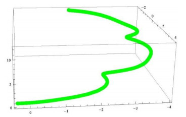
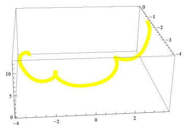
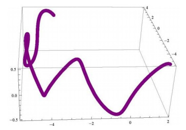
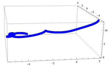
In this paper, adjoint curves generated by means of integral curves of special Smarandache curves with respect to the Bishop frame in three-dimensional Euclidean space were introduced. Relations between the main curve and the Bishop apparatus of these adjoint curves were obtained. Some important results were given concerning the slant helix and general helix of these curves. Finally, these findings were illustrated with figures.
- adjoint curves,
- Smarandache curves,
- general helix,
- slant helix,
- Bishop frame
Citation: Esra Damar. Adjoint curves of special Smarandache curves with respect to Bishop frame[J]. AIMS Mathematics, 2024, 9(12): 35355-35376. doi: 10.3934/math.20241680

Related Papers:

Abstract

In this paper, adjoint curves generated by means of integral curves of special Smarandache curves with respect to the Bishop frame in three-dimensional Euclidean space were introduced. Relations between the main curve and the Bishop apparatus of these adjoint curves were obtained. Some important results were given concerning the slant helix and general helix of these curves. Finally, these findings were illustrated with figures.

References

[1]	L. R. Bishop, There is more than one way to frame a curve, Amer. Math. Month., 82 (1975), 246–251. https://doi.org/10.1080/00029890.1975.11993807 doi: 10.1080/00029890.1975.11993807
[2]	N. Yüksel, A. T. Vanlı, E. Damar, A new approach for geometric properties of DNA structure in $\mathbb{E}$³, Life Sci. J., 12 (2015), 71–79.
[3]	R. S. Millman, G. D. Parker, Elements of differential geometry, Prentice Hall, 1977.
[4]	H.A. Hayden, On a general helix in Riemannian n-space, Proc. London Math. Soc., 32 (1931), 37–45. https://doi.org/10.1112/plms/s2-32.1.337 doi: 10.1112/plms/s2-32.1.337
[5]	M. Barros, General helices and a theorem of Lancret, Proc. Amer. Math. Soc., 125 (1997), 1503–1509.
[6]	S. Izumiya, N. Takeuchi, Special curves and ruled surfaces, Beitrage Algebra Geom., 44 (2003), 203–212.
[7]	S. Izumiya, N. Takeuchi, New special curves and developable surfaces, Turk J. Math., 28 (2004), 153–163.
[8]	B. Bükcü, M. K. Karacan, The slant helices according to Bishop frame, Int. J. Comput. Math. Sci., 3 (2009), 67–70. https://doi.org/10.5281/zenodo.1058229 doi: 10.5281/zenodo.1058229
[9]	J. H. Choi, Y. H. Kim, Associated curves of a Frenet curve and their applications, Appl. Math. Comput., 218 (2012), 9116–9124. https://doi.org/10.1016/j.amc.2012.02.064 doi: 10.1016/j.amc.2012.02.064
[10]	J. H. Choi, Y. H. Kim, A. T. Ali, Some associated curves of Frenet non-lightlike curves in $\mathbb{E}_1.3$, J. Math. Anal. Appl., 394 (2012), 712–723. https://doi.org/10.1016/j.jmaa.2012.04.063 doi: 10.1016/j.jmaa.2012.04.063
[11]	S. Deshmukh, B. Y. Chen, A. Algehanemi, Natural mates of Frenet curves in Euclidean 3-space, Turk. J. Math., 42 (2018), 2826–2840. https://doi.org/10.3906/mat-1712-34 doi: 10.3906/mat-1712-34
[12]	S. K. Nurkan, İ. A. Güven, M. K. Karacan, Characterizations of adjoint curves in Euclidean 3-space, Proc. Natl. Acad. Sci., 89 (2019), 155–161. https://doi.org/10.1007/s40010-017-0425-y doi: 10.1007/s40010-017-0425-y
[13]	D. Canlı, S. Şenyurt, F. E. Kaya, L. Grilli, The pedal curves generated by alternative frame vectors and their Smarandache curves, Symmetry, 16 (2024) 1012. https://doi.org/10.3390/sym16081012
[14]	S. Şenyurt, F. E. Kaya, D. Canlı, Pedal curves obtained from Frenet vector of a space curve and Smarandache curves belonging to these curves, AIMS Math., 9 (2024), 20136–20162. https://doi.org/10.3934/math.2024981 doi: 10.3934/math.2024981
[15]	T. Mendonca, J. Alan, R. Teixeira, Smarandache curves of natural curves pair according to Frenet frame, Adv. Res., 25 (2024), 1–13. https://doi.org/10.9734/air/2024/v25i51131 doi: 10.9734/air/2024/v25i51131
[16]	Y. Li, M. Mak, Framed natural mates of framed curves in Euclidean 3-space, Mathematics, 11 (2023), 3571. https://doi.org/10.3390/math11163571 doi: 10.3390/math11163571
[17]	P. P. Kumar, S. Balakrishnan, S. Magesh, P. Tamizharasi, S. I. Abdelsalam, Numerical treatment of entropy generation and Bejan number into an electroosmotically-driven flow of Sutterby nanofluid in an asymmetric microchannel, Numer. Heat Transfer Part B, 85 (2024), 1–20. https://doi.org/10.1080/10407790.2024.2329773 doi: 10.1080/10407790.2024.2329773
[18]	T. Körpinar, A. Sazak, Optical quantum recursive vortex filament flows and energy with the bishop frame, Opt. Quantum Electron., 55 (2023), 1085. https://doi.org/10.1007/s11082-023-05357-9 doi: 10.1007/s11082-023-05357-9
[19]	N. Yüksel, B. Saltık, E. Damar, Parallel curves in Minkowski 3-space, Gümüşhane Univ. J. Sci. Technol., 12 (2020), 480–486. https://doi.org/10.17714/gumusfenbil.85526519 doi: 10.17714/gumusfenbil.85526519
[20]	M. Turgut, S. Yılmaz, Smarandache curves in Minkowski space time, Int. J. Math. Comb., 3 (2008), 51–55.
[21]	D. Rabouski, F. Smarandache, L. Borisova, Neutrosophic methods in general relativity, APS March Meeting Abstracts, 2018.
[22]	A. T. Ali, Special Smarandache curves in the Euclidean space, Int. J. Math. Comb., 2 (2010), 30–36. https://doi.org/10.5281/ZENODO.9392 doi: 10.5281/ZENODO.9392
[23]	M. Çetin, Y. Tuncer, M. K. Karacan, Smarandache curves according to Bishop frame in Euclidean 3-space, Gen. Math. Notes, 20 (2014), 50–66.
[24]	S. K. Nurkan, İ. Güven, A new approach for Smarandache curves, Turk. J. Math. Comput. Sci., 14 (2022), 155–165. https://doi.org/10.47000/tjmcs.1004423
[25]	S. Şenyurt, A. Çalışkan, Smarandache curves of Mannheim curve couple according to Frenet frame, Math. Sci. Appl. E-Notes, 5 (2017), 122–136. https://doi.org/10.36753/mathenot.421717
[26]	S. Şenyurt, A. Çaliskan, U. Çelik, Smarandache curves of Bertrand curves pair according to Frenet frame, Bol. Soc. Paranaense Mat., 39 (2021), 163–173. https://doi.org/10.5269/bspm.41546
[27]	Y. Altun, C. Cevahir, S. Şenyurt, On the Smarandache curves of spatial quaternionic involute curve, Proc. Natl. Acad. Sci. India Sect. A, 90 (2020) 827–837. https://doi.org/10.1007/s40010-019-00640-5
[28]	S. Şenyurt, Y. Altun, Smarandache curves of the evolute curve according to Sabban frame, Commun. Adv. Math. Sci., 3 (2020), 1–8. https://doi.org/10.33434/cams.594690 doi: 10.33434/cams.594690
[29]	E. M. Solouma, Special equiform Smarandache curves in Minkowski space-time, J. Egypt. Math. Soc., 25 (2017), 319–325. https://doi.org/10.1016/j.joems.2017.04.003 doi: 10.1016/j.joems.2017.04.003
[30]	H. Zhang, Y. Zhao, J. Sun, The geometrical properties of the Smarandache curves on 3-dimension pseudo-spheres generated by null curves, AIMS Math., 9 (2024), 21703–21730. https://doi.org/10.3934/math.20241056 doi: 10.3934/math.20241056
[31]	N. Yüksel, On dual surfaces in Galilean 3-space, AIMS Math., 8 (2023), 4830–4842. https://doi.org/10.3934/math.2023240 doi: 10.3934/math.2023240
[32]	M. Elzawy, S. Mosa, Smarandache curves in the Galilean 4-space G₄, J. Egypt. Math. Soc., 25 (2017), 53–56. https://doi.org/10.1016/j.joems.2016.04.008 doi: 10.1016/j.joems.2016.04.008
[33]	H. S. Abdel-Aziz, M. S. Khalifa, Smarandache curves of some special curves in the Galilean 3-space, Honam Math. J., 37 (2015), 253–264. https://doi.org/10.5831/HMJ.2015.37.2.253 doi: 10.5831/HMJ.2015.37.2.253
[34]	S. Senyurt, D. Canlı, E. Can, S. G. Mazlum, Some special Smarandache ruled surfaces by Frenet frame in E³-Ⅱ, Honam Math. J., 44 (2022), 594–617. https://doi.org/10.5831/HMJ.2022.44.4.594 doi: 10.5831/HMJ.2022.44.4.594
[35]	S. Şenyurt, D. Canlı, E. Çan, S. G. Mazlum, Another application of Smarandache based ruled surfaces with the Darboux vector according to Frenet frame in $\mathbb{E}.3$, Commun. Fac. Sci. Univ. Ankara Ser. A1 Math. Stat., 72 (2023), 880–906. https://doi.org/10.31801/cfsuasmas.1151064 doi: 10.31801/cfsuasmas.1151064
[36]	S. Senyurt, S. G. Mazlum, D. Canli, E. Can, Some special Smarandache ruled surfaces according to alternative frame in E³, Maejo Int. J. Sci. Technol., 17 (2023), 138–153.
[37]	V. Bulut, Adjoint approach between a spatial curve and a ruled surface based on the Bishop frame, Eur. J. Sci. Technol., 34 (2022), 181–192. https://doi.org/10.31590/ejosat.1079225 doi: 10.31590/ejosat.1079225

Reader Comments

Your name:*

Email:*
© 2024 the Author(s), licensee AIMS Press. This is an open access article distributed under the terms of the Creative Commons Attribution License (http://creativecommons.org/licenses/by/4.0)