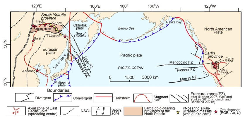
Several similar indicators in Nevada (USA) and South Yakutia (Russia) gold-bearing provinces have been identified based on modern tectonic, geophysical and seismic tomography observations, followed by the analysis of the main geodynamic factors of the formation and distribution of large gold-bearing provinces in the North Pacific. One of the significant metallogenic peculiarities is a wide variety of formational and mineral deposits concentrated in the areas. Both provinces are situated at active margins surrounded by fold-thrust belts. In South Yakutia, a combination of sublatitudinal Baikal-Elkon-Ulkan and submeridional Seligdar-Verkhnetimpon gravity field gradient zones is recorded. In contrast, significant positive gravity anomalies of the Northern Nevada Rift and higher-order gradient zones are presented in Nevada. Large pluton and transform fault zones in both provinces support a conclusion about the fundamental role of geodynamic factors in developing ore-magmatic systems in the regions. Significant differences in the scale of the gold mineralization in the considered provinces are explained by the existence under the North American continent not only of the Mendocino transform fault zone but also of the Juan de Fuca paleo-spreading center. In contrast, the Inagli-Konder-Feklistov magmatic-metallogenic belt alone controls mineralization under the Asian continent.
Citation: Vadim Khomich, Svyatoslav Shcheka, Natalia Boriskina. Geodynamic factors in the formation of large gold-bearing provinces with Carlin-type deposits on continental margins in the North Pacific[J]. AIMS Geosciences, 2023, 9(4): 672-696. doi: 10.3934/geosci.2023036
Several similar indicators in Nevada (USA) and South Yakutia (Russia) gold-bearing provinces have been identified based on modern tectonic, geophysical and seismic tomography observations, followed by the analysis of the main geodynamic factors of the formation and distribution of large gold-bearing provinces in the North Pacific. One of the significant metallogenic peculiarities is a wide variety of formational and mineral deposits concentrated in the areas. Both provinces are situated at active margins surrounded by fold-thrust belts. In South Yakutia, a combination of sublatitudinal Baikal-Elkon-Ulkan and submeridional Seligdar-Verkhnetimpon gravity field gradient zones is recorded. In contrast, significant positive gravity anomalies of the Northern Nevada Rift and higher-order gradient zones are presented in Nevada. Large pluton and transform fault zones in both provinces support a conclusion about the fundamental role of geodynamic factors in developing ore-magmatic systems in the regions. Significant differences in the scale of the gold mineralization in the considered provinces are explained by the existence under the North American continent not only of the Mendocino transform fault zone but also of the Juan de Fuca paleo-spreading center. In contrast, the Inagli-Konder-Feklistov magmatic-metallogenic belt alone controls mineralization under the Asian continent.

| [1] | Muntean JL (2018) Diversity in Carlin-Style Gold Deposits, Reviews in Economic Geology, SEG Inc, 1–363. https://doi.org/10.5382/rev.20 |
| [2] |
Muntean JL, Cline JS, Simon AC, et al. (2011) Magmatic–hydrothermal origin of Nevada's Carlin-type gold deposits. Nature Geosci 4: 122–127. https://doi.org/10.1038/ngeo1064 doi: 10.1038/ngeo1064

|
| [3] | Cline JS, Hofstra AH, Muntean JL, et al. (2005) Carlin-Type Gold Deposits in Nevada: Critical Geologic Characteristics and Viable Models, 100th Anniversary Volume (1905–2005), SEG Inc Econ Geol, 451–484. https://doi.org/10.5382/AV100.15 |
| [4] |
Su WC, Dong WD, Zhang XC, et al. (2018) Carlin-Type Gold Deposits in the Dian-Qian-Gui "Golden Triangle" of Southwest China, In: Muntean JL, Author, Diversity in Carlin-Style Gold Deposits, 157–185. https://doi.org/10.5382/rev.20.05 doi: 10.5382/rev.20.05
|
| [5] | Kim AA (2000) Gold-tellurium-selenium mineralization in Kuranakh Deposit (Central Aldan)[in Russian]. Miner Soc Bull 129: 51–57. |
| [6] | Bakulin YI, Buryak AE, Perestoronin AE (2001) Carlin type gold mineralization (location pattern, genesis, geological basis of forecasting and estimation [in Russian]. DVIMS NRD RF, Khabarovsk. |
| [7] | Vetluzhskikh VG, Kazansky VI, Kochetkov AY, et al. (2002) Central Aldan gold deposits. Geol Ore Deposits 44: 405–434. Available from: https://www.pleiades.online/cgi-perl/search.pl?type = abstract & name = geolore & number = 6 & year = 2 & page = 405. |
| [8] |
Khomich VG, Boriskina NG (2011) Main Geologic-Genetic Types of Bedrock Gold Deposits of the Transbaikal Region and the Russian Far East. Russia. Russ J of Pac Geol 5: 64–84. https://doi.org/10.1134/S1819714011010040 doi: 10.1134/S1819714011010040
|
| [9] |
Khomich VG, Boriskina NG, Santosh M (2014) A geodynamic perspective of world-class gold deposits in East Asia. Gondwana Res 26: 816–833. https://doi.org/10.1016/j.gr.2014.05.007 doi: 10.1016/j.gr.2014.05.007
|
| [10] | Molchanov AV, Terekhov AV, Shatov VV, et al. (2017) Gold ore districts and ore clusters of the Adanian metallogenic province. Reg Geol Metallog 71: 93–111. |
| [11] | Leontev VI, Bushuev YY, Chernigovcev KA (2018) Samolazovskoe gold deposit (Central Aldan ore district): geological structure and mineralization of deep horizons. Reg Geol Metallog 75: 90–103. |
| [12] | Petrov OV, Molchanov AV, Terekhov AV, et al. (2018) Morozkinskoe gold deposit (geological structure and short story of the exploration). Reg Geol Metallog 75: 112–116. Available from: https://elibrary.ru/download/elibrary_36457688_12396066.pdf. |
| [13] |
Minina OV (2019) Paleokarst role in Lebedinsky ore cluster gold orebodies localization, Yakutia[in Russian]. Rudy i Metally 4: 58–74. https://doi.org/10.24411/0869-5997-2019-10032 doi: 10.24411/0869-5997-2019-10032
|
| [14] | Arehart GB, Ressel M, Carne R, et al. (2013) A Comparison of Carlin-type Deposits in Nevada and Yukon. In: Colpron M, Bissig T, Rusk BG, et al., Tectonics, Metallogeny, and Discovery: The North American Cordillera and Similar Accretionary Settings, 389–401. Available from: https://www.segweb.org/store/SearchResults.aspx?Category = SP17-PDF |
| [15] |
Khomich VG, Boriskina NG, Kasatkin SA (2019) Geology, magmatism, metallogeny, and geodynamics of the South Kuril Islands. Ore Geol Rev 105: 151–162. https://doi.org/10.1016/j.oregeorev.2018.12.015 doi: 10.1016/j.oregeorev.2018.12.015
|
| [16] | Grebennikov AV, Khanchuk AI (2021) Geodynamics and magmatism of the pacific-type transform margins. aspects and discriminant diagrams[in Russian]. Tikhookeanskaya Geologiya 40: 3–24. Available from: http://itig.as.khb.ru/POG/2021/n_1/pdf/Grebennikov_RGB.pdf |
| [17] |
Khomich VG, Boriskina NG (2021) Eventual solution to the problems of gold ore trends localization in the Carlin province (Nevada, USA). Int J Earth Sci (Geol Rundsch) 110: 2043–2055. https://doi.org/10.1007/s00531-021-02056-2 doi: 10.1007/s00531-021-02056-2
|
| [18] |
Khomich VG, Boriskina NG (2021) Petroleum potential of the Uchur zone of the Aldan anteclise (Siberian Platform). J Petrol Sci Eng 201: 108501. https://doi.org/10.1016/j.petrol.2021.108501 doi: 10.1016/j.petrol.2021.108501
|
| [19] |
Hronsky JMA, Groves DI, Loucks RR, et al. (2012) A unified model for gold mineralisation in accretionary orogens and implications for regional-scale exploration targeting methods. Miner Deposita 47: 339–358. https://doi.org/10.1007/s00126-012-0402-y doi: 10.1007/s00126-012-0402-y
|
| [20] |
Zhu J, Zhang ZC, Santosh M, et al. (2020) Carlin-style gold province linked to the extinct Emeishan plume. EPSL 530: 115940. https://doi.org/10.1016/j.epsl.2019.115940 doi: 10.1016/j.epsl.2019.115940
|
| [21] | Khanchuk AI (2006) Geodynamics, magmatism, and metallogeny of the Russian East[in Russian]. Dalnauka, Vladivostok. |
| [22] | Hofstra AH, Cline JS (2000) Characteristics and models for Carlin-type gold deposits, In: Hagemann SG, Brow PE, (Eds.), Gold in 2000, 163–220. Available from: https://www.segweb.org/Store/detail.aspx?id = EDOCREV13CH05. |
| [23] | Cline JS (2018) Nevada's Carlin-Type Gold Deposits: What We've Learned During the Past 10 to 15 Years. In: Muntean JL, Diversity in Carlin-Style Gold Deposits, 20: 7–38. https://doi.org/10.5382/rev.20.01 |
| [24] |
Manning AH, Hofstra AH (2017) Noble gas data from Goldfield and Tonopah epithermal Au-Ag deposits, ancestral Cascades Arc, USA: Evidence for a primitive mantle volatile source. Ore Geol Rev 89: 683–700. http://dx.doi.org/10.1016/j.oregeorev.2017.06.023 doi: 10.1016/j.oregeorev.2017.06.023
|
| [25] |
Weil AB, Yonkee WA (2012) Layer-parallel shortening across the Sevier fold-thrust belt and Laramide foreland of Wyoming: spatial and temporal evolution of a complex geodynamic system. EPSL 357–358: 405–420. http://dx.doi.org/10.1016/j.epsl.2012.09.021 doi: 10.1016/j.epsl.2012.09.021
|
| [26] |
Wang J, Li CF (2015) Crustal magmatism and lithospheric geothermal state of western North America and their implications for a magnetic mantle. Tectonophysics 638: 112–125. http://dx.doi.org/10.1016/j.tecto.2014.11.002 doi: 10.1016/j.tecto.2014.11.002
|
| [27] |
Ressel MW, Henry CD (2006) Igneous geology of the Carlin trend, Nevada: development of the Eocene plutonic complex and significance for Carlin-type gold deposits. Econ Geol 101: 347–383. https://doi.org/10.2113/gsecongeo.101.2.347 doi: 10.2113/gsecongeo.101.2.347
|
| [28] | Kuchai VK, Vesson RL (1980) Fixed hot zone, types of orogenesis and Cenozoic tectonics of the USA West. Geotectonics 2: 49–62 |
| [29] | Berger VI, Mosier DL, Bliss JD, et al. (2014) Sediment-hosted gold deposits of the world—Database and grade and tonnage models, Open-File Report 2014–1074. Available from: http://dx.doi.org/10.3133/ofr20141074. |
| [30] | Bray du EA, John DA, Colgan JP, et al. (2019) Morgan, Petrology of Volcanic Rocks Associated with Silver-Gold (Ag-Au) Epithermal Deposits in the Tonopah, Divide, and Goldfield Mining Districts, Nevada. Available from: https://pubs.usgs.gov/sir/2019/5024/sir20195024.pdf. |
| [31] | Fithian MT, Holley EA, Kelly NM (2018) Geology of Gold Deposits at the Marigold Mine, Battle Mountain District, Nevada, In: Muntean JL, Diversity in Carlin-Style Gold Deposits, 121–156. https://doi.org/10.5382/rev.20.04 |
| [32] | Boitsov VE, Pilipenko GN (1998) Gold and uranium in the Mesozoic hydrothermal deposits of the Central Aldan region (Russia)[in Russian]. Geol Ore Deposits 40: 354–369. |
| [33] | Shatova NV, Molchanov AV, Terekhov AV, et al. (2019) Ryabinovoe copper-gold-porphyry deposit (Southern Yakutia): geology, noble gases isotope systematics and isotopic (U-PB, RB-SR, RE-OS) dating of wallrock alteration and ore-forming processes. Regionalnaya Geologiya i Metallogeniya 77: 75–97. Available from: https://elibrary.ru/download/elibrary_37422881_84522683.pdf. |
| [34] |
Van der Meer DG, van Hinsbergen DJJ, Spakmana W (2018) Atlas of the underworld: Slab remnants in the mantle, their sinking history, and a new outlook on lower mantle viscosity. Tectonophysics 723: 309–448. https://doi.org/10.1016/j.tecto.2017.10.004 doi: 10.1016/j.tecto.2017.10.004
|
| [35] | Gainanov AG, Krasny LI, Stroyev PA (1979) Explanatory note to gravimetric maps of the Pacific Ocean and the Pacific Ocean mobile belt [in Russian]. VSEGEI, Leningrad. |
| [36] |
Chen CX, Zhao DP, Wu SG (2015) Tomographic imaging of the Cascadia subduction zone: Constraints on the Juan de Fuca slab. Tectonophysics 647–648: 73–88. http://dx.doi.org/10.1016/j.tecto.2015.02.012 doi: 10.1016/j.tecto.2015.02.012
|
| [37] |
Sigloch K, McQuarrie N, Nolet G (2008) Two-stage subduction history under North America inferred from finite-frequency tomography. Nature Geosci 1: 458–462. https://doi.org/10.1038/ngeo231 doi: 10.1038/ngeo231
|
| [38] |
Faccenna C, Becker W, Lallemand S, et al. (2010) Subduction-triggered magmatic pulses: A new class of plumes? EPSL 299: 54–68. https://doi.org/10.1016/j.epsl.2010.08.012 doi: 10.1016/j.epsl.2010.08.012
|
| [39] |
James DE, Fouch MJ, Carlson RW, et al. (2011) Slab fragmentation, edge flow and the origin of the Yellowstone hotspot track. EPSL 311: 124–135. https://doi.org/10.1016/j.epsl.2011.09.007 doi: 10.1016/j.epsl.2011.09.007
|
| [40] |
Sigloch K (2011) Mantle provinces under North America from multifrequency P wave tomography. Geochem Geophys Geosyst 12: Q02W08. https://doi.org/10.1029/2010GC003421 doi: 10.1029/2010GC003421
|
| [41] | Parfenov LM, Kuzmin MI (2001) Tectonics, geodynamics, and metallogeny of the area of republic of Sakha (Yakutiya)[in Russian]. Nauka, Moscow. |
| [42] | Khomich VG, Boriskina NG (2013) Large gold-ore districts of Southeast Russia: features of position and structure. Lithosphere (Russian). 1: 128–135. Available from: https://elibrary.ru/download/elibrary_19096337_71208627.pdf. |
| [43] | Kazansky VI (2004) The unique Central Aldan gold-uranium ore district (Russia). Geol Ore Deposits 46: 167–181. |
| [44] | Dick IP (1998) Gold placers-giants of Aldan[in Russian]. Otechestvennaya Geologiya 3: 47–49. |
| [45] |
Maximov EP, Nikitin VM, Uyutov VI (2010) The Central Aldan gold-uranium ore magmatogenic system, Aldan-Stanovoy Shield, Russia. Russ J Pac Geol 4: 95–115. https://doi.org/10.1134/S1819714010020016 doi: 10.1134/S1819714010020016
|
| [46] | El'yanov AA, Andreev GV (1991) Magmatism and metallogeny of multistagely activated cratonic areas[in Russian]. Nauka, Novosibirsk. |
| [47] |
Polin VF, Mitsuk VV, Khanchuk AI, et al. (2012) Geochronological limits of subalkaline magmatism in the Ket-Kap-Yuna igneous province, Aldan Shield. Dokl Earth Sci 442: 17–23. https://doi.org/10.1134/S1028334X12010096 doi: 10.1134/S1028334X12010096
|
| [48] | Shatov VV, Molchanov AV, Shatova NV, et al. (2012) Petrography, geochemistry and isotopic (U-Pb and Rb-Sr) dating of alkaline magmatic rocks of the Ryabinovy massif (South Yakutia)[In Russian]. Regionaya Geologiya i Metallogeniya 51: 62–78. |
| [49] | Samovich DA, Tsaruk II, Kokarev AA, et al. (2012) Uranium mineral-raw material base of East Siberia, Irkutsk: Glazkovskaya tipografiya. |
| [50] | Kononova VA, Pervov VA, Bogatikov OA, et al. (1995) Mesozoic potassic magmatism of Central Aldan: geodynamics and genesis[in Russian]. Geotektonika 3: 35–45 |
| [51] | Kazansky VI, Maximov EP, (2000) Geological setting and development history of the El'kon uranium ore district (Aldan Shield, Russia). Geol Ore Deposits 42: 189–204. |
| [52] |
Ponomarchuk AV, Prokop'ev IR, Svetlitskaya TV, et al. (2019) 40Ar/39Ar geochronology of alkaline rocks of the Inagli massif (Aldan Shield, Southern Yakutia). Russ Geol Geophys 60: 33–44. https://doi.org/10.15372/RGG2019003 doi: 10.15372/RGG2019003
|
| [53] | Yanovsky VM, Chmyrev AV, Sorokin AB (1995) Geodynamic Models of Gold in the Regions of Tectono-Magmatic Activization[in Russian]. Rudy i Metally 6: 45–51. |
| [54] | Ibragimova EK, Radkov AV, Molchanov AV, et al. (2015) The results of U-Pb (SHRIMP â…¡) isotope dating of zircons from dunite from massif Inagli (Aldan Shield) and the problem of the genesis of concentrically-oned complexes. Regionalnaya Geologiya i Mmetallogeniya 62: 64–78. Available from: https://elibrary.ru/download/elibrary_24251614_51302773.pdf. |
| [55] | Okrugin AV, Yakubovich OV, Ernst R, et al. (2018) Geology and Mineral Resources of the North-East of Russia[in Russian]. NEFU, Yakutsk. |
| [56] | Khomich VG, Boriskina NG (2016) Essence of the late mesozoic ore-magmatic systems of Aldan Shield. Lithosphere (Russian) 2: 70–90. Available from: https://elibrary.ru/download/elibrary_26008762_33747994.pdf. |
| [57] |
Ronkin YL, Efimov AA, Lepikhina GA, et al. (2013) U-Pb dating of the baddeleytte-zircon system from Pt-bearing dunite of the Konder massif, Aldan Shield: New data. Dokl Earth Sci 450: 607–612. https://doi.org/10.1134/S1028334X13060135 doi: 10.1134/S1028334X13060135
|
| [58] | Kopulov MI (2010) Future views for the gold exploration in the Allakh-Yun metallogenic area, Russian Far East[in Russian]. Otechestvennaya Geologiya 3: 23–32. Available from: https://elibrary.ru/item.asp?id = 14672498. |
| [59] | Shatkov GA, Volsky AS (2004) Tectonics, Deep Structure, and Minerageny of the Amur River Region and Neighboring Areas. Izdatelstvo VSEGEI, St. Petersburg, 1–190. |
| [60] |
Glebovitsky VA, Khil'tova VY, Kozakov IK (2008) tectonics of the Siberian Craton: interpretation of geological, geophysical, geochronological, and isotopic geochemical data. Geotectonics 42: 8–20. https://doi.org/10.1134/S0016852108010020 doi: 10.1134/S0016852108010020
|
| [61] |
Khomich VG, Boriskina NG (2010) Structural position of large gold ore districts in the Central Aldan (Yakutia) and Argun (Transbaikalia) superterranes. Russ Geol Geophys 51: 661–671. https://doi.org/10.1016/j.rgg.2010.05.007 doi: 10.1016/j.rgg.2010.05.007
|
| [62] | Razin LV, Vasyukov VS, Izbekov ED, et al. (1994) Russian Platinum. Developmental problems of mineral and raw materials of platinum metals[in Russian]. Geoinformark, Moscow. |
| [63] | Abramov VA (1995) Deep structure of the Central Aldan region[in Russian]. Dalnauka, Vladivostok. |
| [64] |
Maruyama S, Santosh M, Zhao D (2007) Superplume, supercontinent, and post-perovskite: Mantle dynamics and antiplate tectonics on the Core-Mantle Boundary. Gondwana Res 1: 7–37. http://dx.doi.org/10.1016/j.gr.2006.06.003 doi: 10.1016/j.gr.2006.06.003
|
| [65] |
Zhao D, Pirajno F, Dobretsov NL, et al. (2010) Mantle structure and dynamics under East Russia and adjacent regions. Russ Geol Geophys 51: 925–938. https://doi.org/10.1016/j.rgg.2010.08.003 doi: 10.1016/j.rgg.2010.08.003
|
| [66] |
Koulakov IY, Dobretsov NL, Bushenkova NA, et al (2011) Slab shape in subduction zones beneath the Kurile–Kamchatka and Aleutian arcs based on regional tomography results. Russ Geol Geophys 52: 650–667. https://doi.org/10.1016/j.rgg.2011.05.008 doi: 10.1016/j.rgg.2011.05.008
|
| [67] | Norton IO (2007) Speculations on Cretaceous tectonic history of the northwest Pacific and a tectonic origin for the Hawaii hotspot. GSA Special Papers, The Geological Society of America, 451–470. https://doi.org/10.1130/2007.2430(22) |
| [68] |
Richards JP (2009) Postsubduction porphyry Cu-Au and epithermal Au deposits: Products of remelting of subduction-modified lithosphere. Geology 37: 247–250. https://doi.org/10.1130/G25451A.1 doi: 10.1130/G25451A.1
|


Figures(12)

Vadim Khomich, Svyatoslav Shcheka, Natalia Boriskina. Geodynamic factors in the formation of large gold-bearing provinces with Carlin-type deposits on continental margins in the North Pacific[J]. AIMS Geosciences, 2023, 9(4): 672-696. doi: 10.3934/geosci.2023036


 DownLoad: