Measurement and characterization of infrasound waves from the March 25, 2023 thunderstorm at the near equatorial

Mario Batubara; Masa-yuki Yamamoto; Islam Hosni Hemdan Eldedsouki Hamama; Musthofa Lathif; Ibnu Fathrio; Mario Batubara; Masa-yuki Yamamoto; Islam Hosni Hemdan Eldedsouki Hamama; Musthofa Lathif; Ibnu Fathrio

doi:10.3934/geosci.2023035

AIMS Geosciences

2023, Volume 9, Issue 4: 652-671. doi: 10.3934/geosci.2023035

Previous Article Next Article

Research article

Measurement and characterization of infrasound waves from the March 25, 2023 thunderstorm at the near equatorial

1.
Research Center for Space, National Research and Innovation Agency of Indonesia (BRIN), Indonesia
2.
Kochi University of Technology, Japan
3.
National Research Institute of Astronomy and Geophysics Department of Egyptian, Egypt
4.
Research Center for Climate and Atmosphere, BRIN, Indonesia

Received: 11 July 2023 Revised: 11 September 2023 Accepted: 25 October 2023 Published: 08 November 2023

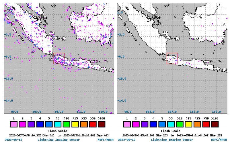
Thunderstorm activity on March 25, 2023 provided a unique opportunity to study the mechanism of lightning events on changes in air pressure. In particular, this event made it possible to study changes in air pressure during thunderstorms using various instruments. This paper presented comprehensive results of infrasound, satellite data, weather radar and weather measurements at the ground during the storm. Observations of lightning events were confirmed using observational data from the International Space Station's Lightning Imaging Sensor (ISS LIS). This work estimated three spectral percentile values on infrasonic sensor data, time series interpolation of standard meteorology profiles, weather radar reflectivity and total radiant energy of lightning from ISS LIS observations during the day and night periods. As a result, during the investigation, it was seen that the recorded infrasound signal in the 0.6–0.8 Hertz (Hz) range was contaminated by background environmental noise, but in the 1–3 Hz band range it was consistent with the appearance of storms that produce high energy blows. Infrasound detection and electromagnetic lightning detection show good correlation up to a distance of 100 km from the infrasonic station. During a thunderstorm, the ISS LIS flight directly above the observation site detected more than 2,000 lightning events. In addition, the application of lightning detection from several independent instruments can provide a complete picture of the observed event.
- infrasound,
- thunderstorm,
- air pressure,
- lightning detection,
- electromagnetic discharge,
- meteorology
Citation: Mario Batubara, Masa-yuki Yamamoto, Islam Hosni Hemdan Eldedsouki Hamama, Musthofa Lathif, Ibnu Fathrio. Measurement and characterization of infrasound waves from the March 25, 2023 thunderstorm at the near equatorial[J]. AIMS Geosciences, 2023, 9(4): 652-671. doi: 10.3934/geosci.2023035

Related Papers:

Abstract

Thunderstorm activity on March 25, 2023 provided a unique opportunity to study the mechanism of lightning events on changes in air pressure. In particular, this event made it possible to study changes in air pressure during thunderstorms using various instruments. This paper presented comprehensive results of infrasound, satellite data, weather radar and weather measurements at the ground during the storm. Observations of lightning events were confirmed using observational data from the International Space Station's Lightning Imaging Sensor (ISS LIS). This work estimated three spectral percentile values on infrasonic sensor data, time series interpolation of standard meteorology profiles, weather radar reflectivity and total radiant energy of lightning from ISS LIS observations during the day and night periods. As a result, during the investigation, it was seen that the recorded infrasound signal in the 0.6–0.8 Hertz (Hz) range was contaminated by background environmental noise, but in the 1–3 Hz band range it was consistent with the appearance of storms that produce high energy blows. Infrasound detection and electromagnetic lightning detection show good correlation up to a distance of 100 km from the infrasonic station. During a thunderstorm, the ISS LIS flight directly above the observation site detected more than 2,000 lightning events. In addition, the application of lightning detection from several independent instruments can provide a complete picture of the observed event.

References

[1]	Lyons JJ, Haney MM, Fee D, et al. (2019) Infrasound from giant bubbles during explosive submarine eruptions. Nat Geosci 12: 952–958. https://doi.org/10.1038/s41561-019-0461-0 doi: 10.1038/s41561-019-0461-0
[2]	Johnson JB, Ripepe M (2011) Volcano infrasound: A review. J Volcanol Geotherm Res 206: 61–69. https://doi.org/10.1016/j.jvolgeores.2011.06.006 doi: 10.1016/j.jvolgeores.2011.06.006
[3]	Fee D, Matoza RS (2013) An overview of volcano infrasound: From hawaiian to plinian, local to global. J Volcanol Geotherm Res 249: 123–139. https://doi.org/10.1016/j.jvolgeores.2012.09.002 doi: 10.1016/j.jvolgeores.2012.09.002
[4]	Matoza RS, Hedlin MAH, Garces MA (2007) An infrasound array study of Mount St. Helens. J Volcanol Geotherm Res 160: 249–262. https://doi.org/10.1016/j.jvolgeores.2006.10.006 doi: 10.1016/j.jvolgeores.2006.10.006
[5]	Matoza RS, Fee D, Garcés MA, et al. (2009) Infrasonic jet noise from volcanic eruptions. Geophys Res Lett 36: L08303. https://doi.org/10.1029/2008GL036486 doi: 10.1029/2008GL036486
[6]	Cook RK (1971) Infrasound Radiated During the Montana Earthquake of 1959 August 18. Geophys J R Astron Soc 26: 191–198. https://doi.org/10.1111/j.1365-246X.1971.tb03393.x doi: 10.1111/j.1365-246X.1971.tb03393.x
[7]	Mutschlecner JP, Whitaker RW (2005) Infrasound from earthquakes. J Geophys Res 110: D01108. https://doi.org/10.1029/2004JD005067 doi: 10.1029/2004JD005067
[8]	Arrowsmith SJ, Whitaker R, Taylor SR, et al. (2008) Regional monitoring of infrasound events using multiple arrays: Application to Utah and Washington State. Geophys J Int 175: 291–300. https://doi.org/10.1111/j.1365-246X.2008.03912.x doi: 10.1111/j.1365-246X.2008.03912.x
[9]	Johnson JB, Mikesell TD, Anderson JF, et al. (2020) Mapping the sources of proximal earthquake infrasound. Geophys Res Lett 47. https://doi.org/10.1029/2020GL091421
[10]	Arrowsmith SJ, Burlacu R, Pankow K, et al. (2012) A seismoacoustic study of the 2011 January 3 Circleville earthquake: Seismoacoustic study: Circleville earthquake. Geophys J Int 189: 1148–1158. https://doi.org/10.1111/j.1365-246X.2012.05420.x doi: 10.1111/j.1365-246X.2012.05420.x
[11]	Le Pichon A, Herry P, Mialle P, et al. (2005) Infrasound associated with 2004–2005 large Sumatra earthquakes and tsunami. Geophys Res Lett 32: L19802. https://doi.org/10.1029/2005GL023893 doi: 10.1029/2005GL023893
[12]	Lin TL, Langston CA (2007) Infrasound from thunder: A natural seismic source. Geophys Res Lett 34: L14304. https://doi.org/10.1029/2007GL030404 doi: 10.1029/2007GL030404
[13]	Chimonas G (1977) A possible source mechanism for mountain-associated infrasound. J Atmos Sci 34: 806–811. https://doi.org/10.1175/1520-0469(1977)034%3C0806:APSMFM%3E2.0.CO;2 doi: 10.1175/1520-0469(1977)034%3C0806:APSMFM%3E2.0.CO;2
[14]	Hupe P (2018) Global infrasound observations and their relation to atmospheric tides and mountain waves. Ph.D. thesis, Ludwig-Maximilians-Universität München, Germany. Available from: https://edoc.ub.uni-muenchen.de/23790/
[15]	Le Pichon A, Ceranna L, Pilger C, et al. (2013) The 2013 Russian fireball large ever detected by CTBTO infrasound sensors. Geophys Res Lett 40: 3732–3737. https://doi.org/10.1002/grl.50619 doi: 10.1002/grl.50619
[16]	Landes M, Ceranna L, Le Pichon A, et al. (2012) Localization of microbarom sources using the IMS infrasound network. J Geophys Res 117: D06102. https://doi.org/10.1029/2011JD016684 doi: 10.1029/2011JD016684
[17]	Arrowsmith SJ, Hedlin, MAH, Stump B, et al. (2008) Infrasonic Signals from Large Mining Explosions. Bull Seismol Soc Amer 98. https://doi.org/10.1785/0120060241
[18]	Bowman DC, Krishnamoorthy S (2021) Infrasound from a buried chemical explosion recorded on a balloon in the lower stratosphere. Geophys Res Lett 48: e2021GL094861. https://doi.org/10.1029/2021GL094861 doi: 10.1029/2021GL094861
[19]	Il-Young Che, Park J, Kim I, et al. (2014) Infrasound signals from the underground nuclear explosions of North Korea. Geophys J Int 198: 495–503. https://doi.org/10.1093/gji/ggu150 doi: 10.1093/gji/ggu150
[20]	Applbaum, D, Averbuch G, Price C, et al. (2019) Infrasound observations of sprites associated with winter thunderstorms in the eastern mediterranean. Atmos Res 235: 104770. https://doi.org/10.1016/j.atmosres.2019.104770 doi: 10.1016/j.atmosres.2019.104770
[21]	Campus P, Christie DR (2010) Worldwide Observations of Infrasonic Waves, In: Le Pichon A, Blanc E, Hauchercorne A. (eds), Infrasound Monitoring for Atmospheric studies, Springer Netherlands, 185–234. https://doi.org/10.1007/978-1-4020-9508-5_6
[22]	Christie DR, Campus P (2010) The IMS Infrasound Network: Design and Establishment of Infrasound Stations, In: Le Pichon A, Blanc E, Hauchercorne A, (eds), Infrasound Monitoring for Atmospheric studies, Springer Netherlands. 29–75. https://doi.org/10.1007/978-1-4020-9508-5_2
[23]	Batubara M, Yamamoto MY (2020) Infrasound Observations of Atmospheric Disturbances Due to a Sequence of Explosive Eruptions at Mt. Shinmoedake in Japan on March 2018. Remote Sens 12: 728. https://doi.org/10.3390/rs12040728
[24]	Houghton HG (1951) On the Physics of Clouds and Precipitation. In: Malone TF, (eds), Compendium of Meteorology. American Meteorological Society, Boston, MA. https://doi.org/10.1007/978-1-940033-70-9_14
[25]	Gaskell W (1981) A laboratory study of the inductive theory of thunderstorm electrification. Quart J Roy Meteor Soc 107: 955–966. https://doi.org/10.1002/qj.49710745413 doi: 10.1002/qj.49710745413
[26]	Gilmore MS, Straka JM, Rasmussen EN (2004) Precipitation and evolution sensitivity in simulated deep convective storms: Comparisons between liquid-only and simple ice and liquid phase microphysics. Mon Weather Rev 132: 1897–1916. https://doi.org/10.1175/1520-0493(2004)132<1897:PAESIS>2.0.CO;2 doi: 10.1175/1520-0493(2004)132<1897:PAESIS>2.0.CO;2
[27]	Jayaratne ER, Saunders CPR (1985) Thunderstorm electrification: The effect of cloud droplets. J Geophys Res 90: 13063–13066. https://doi.org/10.1029/JD090iD07p13063 doi: 10.1029/JD090iD07p13063
[28]	Lang TJ, Jay Miller L, Weisman M, et al. (2004) The Severe Thunderstorm Electrification and Precipitation Study. Bull Amer Meteor Soc 85: 1107–1126. https://doi.org/10.1175/BAMS-85-8-1107 doi: 10.1175/BAMS-85-8-1107
[29]	Pereyra RG, Avila EE, Castellano NE, et al. (2000) A laboratory study of graupel charging. J Geophys Res 105: 20803–20812. https://doi.org/10.1029/2000JD900244 doi: 10.1029/2000JD900244
[30]	Qie X, Yuan S, Chen Z, et al. (2021) Understanding the dynamical-microphysical-electrical processes associated with severe thunderstorms over the Beijing metropolitan region. Sci China Earth Sci 64: 10–26. https://doi.org/10.1007/s11430-020-9656-8 doi: 10.1007/s11430-020-9656-8
[31]	Reynolds SE, Brook M, Gourley MF (1957) Thunderstorm charge separation. J Atmos Sci 14: 426–436. https://doi.org/10.1175/1520-0469(1957)014<0426:TCS>2.0.CO;2 doi: 10.1175/1520-0469(1957)014<0426:TCS>2.0.CO;2
[32]	Saunders CPR (1993) A review of thunderstorm electrification processes. J Appl Meteor Climatol 32: 642–655. https://doi.org/10.1175/1520-0450(1993)032<0642:AROTEP>2.0.CO;2 doi: 10.1175/1520-0450(1993)032<0642:AROTEP>2.0.CO;2
[33]	Takahashi T (1978) Riming electrification as a charge generation mechanism in thunderstorms. J Atmos Sci 35: 1536–1548. https://doi.org/10.1175/1520-0469(1978)035<1536:REAACG>2.0.CO;2 doi: 10.1175/1520-0469(1978)035<1536:REAACG>2.0.CO;2
[34]	Wang X, Liao R, Li J, et al. (2020) Thunderstorm identification algorithm research based on simulated airborne weather radar reflectivity data. J Wireless Com Network 37. https://doi.org/10.1186/s13638-020-1651-6
[35]	Petersen WA, Rutledge SA (1998) On the relationship between cloud-to-ground lightning and convective rainfall. J Geophys Res 103: 14025–14040. https://doi.org/10.1029/97JD02064 doi: 10.1029/97JD02064
[36]	Price C, Federmesser B (2006) Lightning-rainfall relationships in Mediterranean winter thunderstorms. Geophys Res Lett 33: L07813. https://doi.org/10.1029/2005GL024794 doi: 10.1029/2005GL024794
[37]	Blakeslee R, Koshak W (2016) LIS on ISS: Expanded Global Coverage and Enhanced Applications. Earth Obs 28: 4–14.
[38]	Blakeslee RJ, Lang TJ, Koshak WJ, et al. (2020) Three Years of the Lightning Imaging Sensor Onboard the International Space Station: Expanded Global Coverage and Enhanced Applications. J Geophys Res Atmos 125: e2020JD032918. https://doi.org/10.1029/2020JD032918 doi: 10.1029/2020JD032918
[39]	Baldini L, Roberto N, Montopoli M, et al. (2018) Ground-Based Weather Radar to Investigate Thunderstorms. In: Andronache C, (eds), Remote Sensing of Clouds and Precipitation. Springer Remote Sensing/Photogrammetry. Springer, Cham. https://doi.org/10.1007/978-3-319-72583-3_4
[40]	Hwang SH, Kim KB, Han D (2020) Comparison of methods to estimate areal means of short duration rainfalls in small catchments, using rain gauge and radar data. J Hydrol 588: 125084. https://doi.org/10.1016/j.jhydrol.2020.125084 doi: 10.1016/j.jhydrol.2020.125084
[41]	Prajapati R, Silwal P, Duwal S, et al. (2022) Detectability of rainfall characteristics over a mountain river basin in the Himalayan region from 2000 to 2015 using ground-and satellite-based products. Theor Appl Climatol 147: 185–204. https://doi.org/10.1007/s00704-021-03820-9 doi: 10.1007/s00704-021-03820-9
[42]	Wu F, Cui X, Zhang DL, et al. (2017) The relationship of lightning activity and short-duration rainfall events during warm seasons over the Beijing metropolitan region. Atmos Res 195: 31–43. https://doi.org/10.1016/j.atmosres.2017.04.032 doi: 10.1016/j.atmosres.2017.04.032
[43]	Williams E, Mkrtchyan H, Mailyan B, et al. (2022) Radar diagnosis of the thundercloud electron accelerator. J Geophys Res Atmos 127: e2021JD035957. https://doi.org/10.1029/2021JD035957 doi: 10.1029/2021JD035957
[44]	Uman MA (2001) The lightning discharges, Courier Corporation.
[45]	Rakov VA, Uman MA (2003) Lightning, Physics and Effects, Cambridge University Press, New York. 687. https://doi.org/10.1017/CBO9781107340886
[46]	Few AA, Teer TL (1974) The accuracy of acoustic reconstructions of lightning channels. J Geophys Res 79: 5007–5011. https://doi.org/10.1029/JC079i033p05007 doi: 10.1029/JC079i033p05007
[47]	MacGorman DR, Few AA, Teer TL (1981) Layered lightning activity. J Geophys Res 86: 9900–9910. https://doi.org/10.1029/JC086iC10p09900 doi: 10.1029/JC086iC10p09900
[48]	Hagenguth JH (1951) The Lightning Discharge. In: Malone TF, Eds., Compendium of Meteorology. American Meteorological Society, Boston, MA. https://doi.org/10.1007/978-1-940033-70-9_11
[49]	Dessler AJ (1973) Infrasonic thunder. J Geophys Res 78: 1889–1896. https://doi.org/10.1029/JC078i012p01889 doi: 10.1029/JC078i012p01889
[50]	Pasko VP (2009) Mechanism of lightning associated infrasonic pulses from thunderclouds. J Geophys Res 114: D08205. https://doi.org/10.1029/2008JD011145 doi: 10.1029/2008JD011145
[51]	Liszka L (2004) On the possible infrasound generation by sprites. J Low Freq Noise V A 23: 85–93. https://doi.org/10.1260/0263092042869838 doi: 10.1260/0263092042869838
[52]	Farges T, Blanc E, le Pichon A, et al. (2005) Identification of infrasound produced by sprites during the Sprite2003 campaign. Geophys Res Lett 32: L01813. https://doi.org/10.1029/2004GL021212 doi: 10.1029/2004GL021212
[53]	Liszka L, Hobara Y (2006) Sprite-attributed infrasonic chirps—Their detection, occurrence and properties between 1994 and 2004. J Atmos Solar-Terr Phys 68: 1179–1188. https://doi.org/10.1016/j.jastp.2006.02.016 doi: 10.1016/j.jastp.2006.02.016
[54]	Blanc E (1985) Observations in the upper atmosphere of infrasonic waves from natural or artificial sources: A summary. Ann Geophys 3: 673–688.
[55]	Few AA (1995) Acoustic radiations from lightning. Handbook of Atmospheric Electrodynamics, CRC Press, Boca Raton, 1–31. https://doi.org/10.1201/9780203713297
[56]	Drob DP, Picone JM, Garces M (2003) Global morphology of infrasound propagation. J Geophys Res 108: 4680. https://doi.org/10.1029/2002JD003307 doi: 10.1029/2002JD003307
[57]	Nugroho GA, Sinatra T, Fathrio I (2018) Application of rain scanner SANTANU and transportable weather radar in analyze of Mesoscale Convective System (MCS) events over Bandung, West Java. IOP Conf Ser Earth Environ Sci 149: 012058. https://iopscience.iop.org/article/10.1088/1755-1315/149/1/012058
[58]	Zel'dovich YB, Raizer YP (2002) Physics of shock waves and high-temperature hydrodynamic phenomena, Academic Press, New York & London.
[59]	Few AA (1982) Acoustic radiations from lightning. Handbook of Atmospherics, CRC Press, Inc., Boca Raton, 257–289.
[60]	Few AA (1985) The production of lightning-associated infrason ic acoustic sources in thunderclouds. J Geophys Res 90: 6175–6180. https://doi.org/10.1029/JD090ID04P06175 doi: 10.1029/JD090ID04P06175

geosci-09-04-035-s001.zip

Reader Comments

Your name:*

Email:*
© 2023 the Author(s), licensee AIMS Press. This is an open access article distributed under the terms of the Creative Commons Attribution License (http://creativecommons.org/licenses/by/4.0)