Evaluating the impact of multiple factors on the control of COVID-19 epidemic: A modelling analysis using India as a case study

Aili Wang; Xueying Zhang; Rong Yan; Duo Bai; Jingmin He; Aili Wang; Xueying Zhang; Rong Yan; Duo Bai; Jingmin He

doi:10.3934/mbe.2023269

Mathematical Biosciences and Engineering

2023, Volume 20, Issue 4: 6237-6272. doi: 10.3934/mbe.2023269

Previous Article Next Article

Research article Special Issues

Evaluating the impact of multiple factors on the control of COVID-19 epidemic: A modelling analysis using India as a case study

1.
School of Science, Xi'an University of Technology, Xi'an 710054, China
2.
School of Mathematics and Information Science, Baoji University of Arts and Sciences, Baoji 721013, China

Academic Editor: Xiaodi Li

Received: 23 September 2022 Revised: 10 January 2023 Accepted: 11 January 2023 Published: 31 January 2023

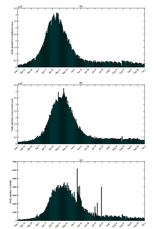
The currently ongoing COVID-19 outbreak remains a global health concern. Understanding the transmission modes of COVID-19 can help develop more effective prevention and control strategies. In this study, we devise a two-strain nonlinear dynamical model with the purpose to shed light on the effect of multiple factors on the outbreak of the epidemic. Our targeted model incorporates the simultaneous transmission of the mutant strain and wild strain, environmental transmission and the implementation of vaccination, in the context of shortage of essential medical resources. By using the nonlinear least-square method, the model is validated based on the daily case data of the second COVID-19 wave in India, which has triggered a heavy load of confirmed cases. We present the formula for the effective reproduction number and give an estimate of it over the time. By conducting Latin Hyperbolic Sampling (LHS), evaluating the partial rank correlation coefficients (PRCCs) and other sensitivity analysis, we have found that increasing the transmission probability in contact with the mutant strain, the proportion of infecteds with mutant strain, the ratio of probability of the vaccinated individuals being infected, or the indirect transmission rate, all could aggravate the outbreak by raising the total number of deaths. We also found that increasing the recovery rate of those infecteds with mutant strain while decreasing their disease-induced death rate, or raising the vaccination rate, both could alleviate the outbreak by reducing the deaths. Our results demonstrate that reducing the prevalence of the mutant strain, improving the clearance of the virus in the environment, and strengthening the ability to treat infected individuals are critical to mitigate and control the spread of COVID-19, especially in the resource-constrained regions.

Keywords:

Citation: Aili Wang, Xueying Zhang, Rong Yan, Duo Bai, Jingmin He. Evaluating the impact of multiple factors on the control of COVID-19 epidemic: A modelling analysis using India as a case study[J]. Mathematical Biosciences and Engineering, 2023, 20(4): 6237-6272. doi: 10.3934/mbe.2023269

Related Papers:

[1]	Keqiang Li, Shangjiu Wang . Multiple periodic solutions of nonlinear second order differential equations. AIMS Mathematics, 2023, 8(5): 11259-11269. doi: 10.3934/math.2023570
[2]	Wangjin Yao . Variational approach to non-instantaneous impulsive differential equations with $p$ -Laplacian operator. AIMS Mathematics, 2022, 7(9): 17269-17285. doi: 10.3934/math.2022951
[3]	Yuhua Long, Sha Li . Results on homoclinic solutions of a partial difference equation involving the mean curvature operator. AIMS Mathematics, 2025, 10(3): 6429-6447. doi: 10.3934/math.2025293
[4]	Liuyang Shao, Haibo Chen, Yicheng Pang, Yingmin Wang . Multiplicity of nontrivial solutions for a class of fractional Kirchhoff equations. AIMS Mathematics, 2024, 9(2): 4135-4160. doi: 10.3934/math.2024203
[5]	Minggang Xia, Xingyong Zhang, Danyang Kang, Cuiling Liu . Existence and concentration of nontrivial solutions for an elastic beam equation with local nonlinearity. AIMS Mathematics, 2022, 7(1): 579-605. doi: 10.3934/math.2022037
[6]	Andrey Muravnik . Nonclassical dynamical behavior of solutions of partial differential-difference equations. AIMS Mathematics, 2025, 10(1): 1842-1858. doi: 10.3934/math.2025085
[7]	D. Fernández-Ternero, E. Macías-Virgós, D. Mosquera-Lois, N. A. Scoville, J. A. Vilches . Fundamental theorems of Morse theory on posets. AIMS Mathematics, 2022, 7(8): 14922-14945. doi: 10.3934/math.2022818
[8]	Muhammad Sarwar, Aiman Mukheimer, Syed Khayyam Shah, Arshad Khan . Existence of solutions of fractal fractional partial differential equations through different contractions. AIMS Mathematics, 2024, 9(5): 12399-12411. doi: 10.3934/math.2024606
[9]	Yuhua Long . Existence of two homoclinic solutions for a nonperiodic difference equation with a perturbation. AIMS Mathematics, 2021, 6(5): 4786-4802. doi: 10.3934/math.2021281
[10]	Jun Lei, Hongmin Suo . Multiple solutions of Kirchhoff type equations involving Neumann conditions and critical growth. AIMS Mathematics, 2021, 6(4): 3821-3837. doi: 10.3934/math.2021227

Abstract

1. Introduction

1.1. Overview

Many physical phenomena, in the fields of sound and electrical waves, heat transfer, mechanics, and optics can be described through partial differential equations. Therefore, we can say that the study of mathematical physics depends primarily on the study of partial differential equations. During previous decades, many methods were developed to reduce and solve partial differential equations, including Symmetry method ^[1,2,3,4], scattering transformation ^[5], Tanh method ^[6], the homogeneous balance method ^[7], Aboodh transform decomposition method ^[8], ( $G^{\prime}/G$ , $1/G$ )-expansion method ^[9], Exp-function method ^[10], Generalized He's Exp-function method ^[11], Kudryashov method ^[12], and Generalized Kudryashov method ^[13]. Consider the nonlinear (2+1)-dimensional Date-Jimbo-Kashiwara-Miwa (DJKM) equation ^[14,15] in the following form:

$\begin{equation} \Phi_{xxxxy}+4\Phi_{xxy}\Phi_{x}+2\Phi_{xxx}\Phi_{y}+6\Phi_{xy}\Phi_{xx} +\Phi_{yyy}-2\Phi_{xxt} = 0, \end{equation}$

(1)

where $\Phi = \Phi(x, y, t).$ DJKM describes the wave diffusion of physical-quantity, and it has certain applications in plasma physics ^[16,17]. This equation was presented by Jimbo and Miwa as second formulas for Kadomtsev-Petviashvili hierarchy.

1.2. Related literatures

There is a wealth of literature related to this governing equation such as: Bibi and Ahmad ^[14] who employed the symmetry method to reduce the governing equation to another equation of lower order and obtained its exact solutions. The exp( $-\phi$ ( $\xi$ ))-Expansion Method was utilized by Sajid and Akram ^[14] for obtaining traveling wave solutions for Eq (1). Halder et al. ^[18] used the Lie symmetry analysis and singularity method to study one type of the governing equation. Wazwaz ^[19] studied the integrability of this equation and obtained multiple soliton solutions by using Painlevé analysis and Hirota's method. Akram et al. ^[16] applied the extended direct algebraic method to obtain exact solutions for the governing equation.

1.3. Main idea

The previous literature led us to determine the study of the governing equation to apply the Lie symmetry method and the Generalized Kudryashov method. Our main objective of this paper is to convert the governing equation to several distinct ordinary differential equations (ODE). We then solve the resulting ODEs to obtain exact and novel wave solutions for the governing equation. As a result, we can show the dynamic behavior of wave solutions in 2-D and 3-D plots.

2. Lie symmetry method

In this part, the Lie symmetry method ^[20,21,22] is used to deduce the similarity reductions for the governing equation, so the one-parameter Lie symmetry of infinitesimal variables is shown as follows:

$\begin{align*} t^{\ast} & = t+\varepsilon A(t,x,y,\Phi)+o(\varepsilon^{2}),\text{ }x^{\ast } = x+\varepsilon B(t,x,y,\Phi)+o(\varepsilon^{2}),\nonumber\\ y^{\ast} & = y+\varepsilon C(t,x,y,\Phi)+o(\varepsilon^{2}),\text{ } \Phi^{\ast} = \Phi+\varepsilon E(t,x,y,\Phi)+o(\varepsilon^{2}), \end{align*}$

(2)

where $\varepsilon$ is the one parameter Lie group, $A, \; B, \; C$ and $E$ are infinitesimal variables and $t, \; x$ and $y$ are independent variables of the function $\Phi.$

The vector generator $\chi$ is related to the above-mentioned group transformations which can be written as the following expression:

$\begin{equation} \chi = A\frac{\partial}{\partial t}+B\frac{\partial}{\partial x}+C\frac {\partial}{\partial y}+E\frac{\partial}{\partial\Phi}, \end{equation}$

(3)

when the following invariance condition is satisfied:

$\begin{equation} \Gamma^{(3)}(\Delta) = 0, \end{equation}$

(4)

where $\Delta$ represents Eq (1) and $\Gamma^{(3)}$ is the third order prolongation^[23,24] of the operator V

$\begin{align*} \Gamma^{(3)} & = \chi+E_{[x]}\frac{\partial}{\partial\Phi_{x}}+E_{[y]} \frac{\partial}{\partial\Phi_{y}}+E_{[xy]}\frac{\partial}{\partial\Phi_{xy} }+E_{[xxx]}\frac{\partial}{\partial\Phi_{xxx}}+E_{[xxy]}\frac{\partial }{\partial\Phi_{xxy}}\nonumber\\ & +E_{[xxt]}\frac{\partial\Phi}{\partial\Phi_{xxt}}+E_{[xxy]}\frac{\partial }{\partial\Phi_{xxy}}+E_{[xxxy]}\frac{\partial}{\partial\Phi_{xxxy}} +E_{[yyy]}\frac{\partial}{\partial\Phi_{yyy}}, \end{align*}$

(5)

where the components $E_{[x]}, E_{[xx]}, \; E_{[xyy]}, \; E_{[y]}, \; E_{[xy]}....$ can be determined from the following expressions:

$\begin{align*} E_{[x]} & = D_{x}E-\Phi_{t}D_{x}A-\Phi_{x}D_{x}B-\Phi_{y}D_{x}C,\nonumber\\ E_{[y]} & = D_{y}E-\Phi_{t}D_{y}A-\Phi_{x}D_{y}B-\Phi_{y}D_{y}C,\nonumber\\ \text{ }E_{[xx]} & = D_{x}E_{[x]}-\Phi_{xt}D_{x}A-\Phi_{xx}D_{x}B-\Phi _{xy}D_{x}C,\nonumber\\ \text{ }E_{[xy]} & = D_{y}E_{[x]}-\Phi_{xt}D_{y}A-\Phi_{xx}D_{y}B-\Phi _{xy}D_{y}C,\nonumber\\ \text{ }E_{[yy]} & = D_{y}E_{[y]}-\Phi_{xt}D_{y}A-\Phi_{xx}D_{y}B-\Phi _{xy}D_{y}C,\nonumber\\ E_{[xxxy]} & = D_{y}E_{[xxx]}-\Phi_{xxxt}D_{y}A-\Phi_{xxxx}D_{y}B-\Phi _{xxxy}D_{y}C. \end{align*}$

(6)

Substituting (1) into Eq (4), yields an identity components $A_{x}, A_{xx}, \; B_{t}, B_{x}, ....$ and adding the coefficients of $\Phi_{x, x, t}$ , $\Phi_{y, y, y}$ , ... and equating them to zero, then the infinitesimals $A, B, C$ and $E$ are obtained from the following equations:

$A_{x} = A_{y} = A_{\Phi} = 0,$

$B_{y} = B_{\Phi} = 0,B_{x} = \frac{1}{4}A_{t},$

$C_{x} = B_{\Phi} = 0,\text{ }C_{z} = \frac{1}{2}A_{t},$

$\begin{equation} E_{x} = \frac{-1}{2}C_{t},\text{ }E_{\Phi} = \frac{-1}{4}A_{t},\text{ }E_{y} = \frac{-1}{2}B_{t}. \end{equation}$

(7)

solving the system of Eq (7), we get

$\begin{align*} A & = g_{1}(t),\text{ }B = \frac{1}{4}g_{1}^{\prime}x+g_{3}(t),\text{ }C = \frac{1}{2}g_{1}^{\prime}y+g_{2}(t),\text{ }\nonumber\\ E & = \frac{-1}{4}g_{1}^{\prime}\Phi-\frac{1}{4}xyg_{1}^{\prime\prime} -yg_{2}^{\prime}-\frac{1}{2}xg_{3}^{\prime}+g_{4}(t). \end{align*}$

(8)

The vector field operator $V$ of Eq (8) can be presented as

$\begin{equation} V = V_{1}(c_{1})+V_{2}(c_{2})+V_{3}(c_{3})+V_{4}(c_{4}), \end{equation}$

(9)

where

$\begin{align*} V_{1} & = g_{1}(t)\left( \frac{\partial}{\partial t}+\frac{1}{4} x\frac{\partial}{\partial x}+\frac{1}{2}y\frac{\partial}{\partial y}-\frac {1}{4}\Phi\frac{\partial}{\partial\Phi}\right) -\frac{1}{4}xyg_{1} ^{\prime\prime}\frac{\partial}{\partial\Phi},\nonumber\\ V_{2} & = g_{2}(t)\frac{\partial}{\partial y}-y\alpha_{2}^{\prime} \frac{\partial}{\partial\Phi},\text{ }V_{3} = g_{3}(t)\frac{\partial }{\partial x}-\frac{1}{2}g_{3}^{\prime}\frac{\partial}{\partial\Phi},\text{ }V_{4} = g_{4}(t)\frac{\partial}{\partial\Phi}. \end{align*}$

(10)

The Lie-bracket $[V_{i}, V_{j}] = V_{i}V_{j}-V_{j}V_{i}$ is used for obtaining the commutator relations which are shown in Table 1, where

$\begin{align*} l_{1} & = g_{1}g_{2}^{\prime}-\frac{1}{2}g_{2}g_{1}^{\prime},\text{ } l_{2} = \frac{-1}{4}(g_{2}^{\prime}g_{1}^{\prime}+2g_{1}g_{2}^{\prime\prime }-g_{2}g_{1}^{\prime\prime})x,\nonumber\\ l_{3} & = g_{1}g_{3}^{\prime}-\frac{1}{4}g_{3}g_{1}^{\prime},\text{ } l_{4} = \frac{-1}{4}(g_{3}^{\prime}g_{1}^{\prime}+4g_{1}g_{3}^{\prime\prime }-g_{3}g_{1}^{\prime\prime})y,\nonumber\\ l_{5} & = \frac{1}{4}(4g_{1}g_{4}^{\prime}+g_{4}g_{1}^{\prime}),\text{ } l_{6} = \frac{-1}{2}(2g_{2}g_{3}^{\prime}-g_{3}g_{2}^{\prime}). \end{align*}$

(11)

Table 1. The commutator table.

	$V_{1}$	$V_{2}$	$V_{3}$	$V_{4}$
$V_{1}$	$0$	$l_{1}\frac{\partial}{\partial y}+l_{2}\frac{\partial }{\partial\Phi}$	$l_{3}\frac{\partial}{\partial x}+a_{4}\frac{\partial }{\partial\Phi}$	$l_{5}\frac{\partial}{\partial\Phi}$
$V_{2}$	-( $l_{1}\frac{\partial}{\partial y}+l_{2}\frac{\partial} {\partial\Phi})$	$0$	$l_{6}\frac{\partial}{\partial\Phi}$	$0$
$V_{3}$	-( $l_{3}\frac{\partial}{\partial x}+l_{4}\frac{\partial} {\partial\Phi})$	- $l_{6}\frac{\partial}{\partial\Phi}$	$0$	$0$
$V_{4}$	$-l_{5}\frac{\partial}{\partial\Phi}$	- $l_{6}\frac{\partial }{\partial\Phi}$	$0$	$0$

| Show Table

DownLoad: CSV

3. Reductions and closed form solutions

To obtain new independent variables, we utilize the characteristic equation as follows:

$\begin{equation} \frac{dt}{A(t,x,y,\Phi)} = \frac{dx}{B(t,x,y,\Phi)} = \frac{dy}{C(t,x,y,\Phi )} = \frac{d\Phi}{E(t,x,y,\Phi)}. \end{equation}$

(12)

Case I. Using $V_{1}$ where $g_{1}(t) = t^{2},$ Eq (12) takes the following form:

$\begin{equation} \frac{dt}{t^{2}} = \frac{dx}{\frac{1}{2}tx} = \frac{dy}{ty} = \frac{d\Phi}{\frac {-1}{2}t\Phi}. \end{equation}$

(13)

The similarity solution of Eq (1) takes the form

$\begin{equation} \Phi(t,x,y) = \frac{1}{\sqrt{t}}F(\zeta,\eta)-\frac{xy}{2t}, \end{equation}$

(14)

where $\zeta = \frac{x}{\sqrt{t}}, \; \eta = \frac{y}{t}.$ Substituting $\Phi$ in Eq (1) we get

$\begin{equation} F_{\eta\eta\eta}+6F_{\zeta\zeta}F_{\zeta\eta}+2F_{\zeta\zeta\zeta }F_{\eta}+4F_{\zeta\zeta\eta}F_{\zeta}+F_{\zeta\zeta\zeta\zeta\eta } = 0. \end{equation}$

(15)

The ordinary differential equations of Eq (15) take the following experssion:

$\begin{equation} h^{3}F^{\prime\prime\prime}(\theta)+6k^{3}hF^{\prime\prime^{2}}(\theta )+6k^{3}hF^{\prime\prime\prime}(\theta)F^{\prime}(\theta)+k^{4}hF^{\prime \prime\prime\prime\prime}(\theta) = 0, \end{equation}$

(16)

where $\theta = k\zeta+h\eta.$

To obtain the exact solution for Eq (16), we utilize generalized Kudryashov method (GKM) ^[11], given as follows:

$\begin{equation} F(\theta) = A_{0}+\sum\limits_{i=1}^m\frac{A_{i}}{(1+\phi (\theta))^{i}}, \end{equation}$

(17)

where $\phi(\theta)$ is the solution for the following Ricati equation $\phi^{\prime}(\theta) = A+B\phi(\theta)+C\phi^{2}(\theta).$ For simplicity, we take $i = 1$ and substitute Eq (17) into Eq (16) then to obtain

$\begin{equation} h = \pm\sqrt{4AC-B^{2}}k^{2},\text{ }A_{1} = 2k(C-B+A),\text{ }k\text{ and }A_{0}\text{ are arbitrary constant.} \end{equation}$

(18)

Substituting Eq (18) into Eqs (14) and (17), the exact solutions of Eq (1) can be expressed as

Set 1. $A\neq0, B\neq0, C\neq0.$

$\begin{equation} \Phi(t,x,y) = \frac{1}{\sqrt{t}}\left( A_{0}+\frac{2k(C-B+A)}{{\Large [} \frac{-B}{2C}\text{+}\frac{\sqrt{4AC-B^{2}}}{2C}\tan\text{(}\frac{1} {2}\text{(}\sqrt{4AC-B^{2}}\theta\text{))}+1{\LARGE ]}}\right) -\frac{xy} {2t}, \end{equation}$

(19)

where $\theta = k\frac{x}{\sqrt{t}}+\sqrt{4AC-B^{2}}k^{2}\frac{y}{t}.$

Set 2. $A = \frac{-1}{2}, B = 0, C = \frac{-1}{2}.$

$\begin{equation} \Phi(t,x,y) = \frac{1}{\sqrt{t}}\left( A_{0}+\frac{-2k}{\cot(\theta)\pm \csc(\theta)+1}\right) -\frac{xy}{2t}, \end{equation}$

(20)

where $\theta = k\frac{x}{\sqrt{t}}+2k^{2}\frac{y}{t}.$

Case II. Substituting $V_{1}$ in Eq (12) where $g_{1}(t) = t,$ then Eq (12) is expressed as follows:

$\begin{equation} \frac{dt}{t} = \frac{dx}{\frac{1}{4}x} = \frac{dy}{\frac{1}{2}y} = \frac{d\Phi }{\frac{-1}{4}\Phi}. \end{equation}$

(21)

Then the invariants are presented by $\zeta = \frac{x}{t^{\frac{1}{4}}}, \; \eta = \frac{y}{t^{\frac{1}{2}}}$ and $\Phi(t, x, y) = \frac{1}{t^{\frac{1}{4}} }F(\zeta, \eta).$ Further Eq (1) is reduced to the following form:

$\begin{align*} \frac{3}{2}F_{\zeta\zeta}+\frac{1}{2}\zeta F_{\zeta\zeta\zeta}+\eta F_{\eta\eta\eta}+F_{\eta\eta\eta}+6F_{\zeta\zeta}F_{\zeta\eta}+ 4F_{\zeta}F_{\zeta\zeta\eta}+2F_{\zeta\zeta\zeta}F_{\eta}+F_{\zeta \zeta\zeta\zeta\eta} = 0. \end{align*}$

(22)

For reducing Eq (22) to ODE we have two subcases:

Subcase (a). Using the scaling transformation in Eq (22)

$\begin{equation} F = e^{\epsilon}\text{ }\overset{-}{F},\text{ }\zeta = e^{\epsilon_{1}}\text{ }\overset{-}{\zeta},\text{ }\eta = e^{\epsilon_{2}}\text{ }\eta. \end{equation}$

(23)

Substituting from Eq (23) into Eq (22) we have $2\epsilon_{1} = \epsilon _{2} = -2\epsilon.$

The characteristic is given as

$\begin{equation} \frac{2d\zeta}{\zeta} = \frac{d\eta}{\eta} = \frac{-2dF}{F}. \end{equation}$

(24)

The invariant variables can be written as

$\begin{equation} \theta = \frac{\zeta^{2}}{\eta},\text{ }f = \frac{1}{\zeta^{2}}F(\theta). \end{equation}$

(25)

The ODE of Eq (22) is provided by

$\begin{align*} -\theta^{2}f^{\prime\prime\prime}-6f^{\prime\prime}-6\theta f^{\prime }-48\theta f^{\prime\prime^{2}}-48\theta ff^{\prime}-48f^{\prime} f^{\prime\prime\prime}-16f^{\prime}f^{\prime\prime\prime}-80\theta f^{\prime\prime\prime} -60f^{\prime\prime\prime}-16\theta^{2}f^{\prime\prime\prime\prime\prime} = 0. \end{align*}$

(26)

To obtain the exact solutions of Eq (26), we suppose that the solution of Eq (26) has the form

$\begin{equation} f(\theta) = A_{0}+\sum\limits_{j=1}^nA_{j}\theta^{j}. \end{equation}$

(27)

For simplicity, we take $j = 2$ , substitute Eq (27) into Eq (26), then the closed form solution of Eq (1) takes the expression

$\begin{equation} \Phi(x,y) = A_{0}+A_{1}\frac{x}{y}-\frac{1}{16}\frac{x^{3}}{y^{2}}, \end{equation}$

(28)

where $A_{0}$ and $A_{1}$ are arbitrary constant.

Subcase (b). Utilizing symmetry method for Eq (22), we obtained the infinitesimals of Eq (22) as follows:

$\begin{equation} \tau = \frac{1}{2}c_{1}\zeta+c_{2},\text{ }\beta = c_{1}\eta+c_{3},\text{ }\psi = \frac{-1}{2}(F+xy)c_{1}-\frac{1}{4}\eta c_{2}-\frac{1}{4}\zeta c_{3}. \end{equation}$

(29)

The vector field of Eq (22) can take the form

$\begin{equation} \chi = \chi_{1}(c_{1})+\chi_{2}(c_{2})+\chi_{3}(c_{3}), \end{equation}$

(30)

where

$\begin{equation} \chi_{1} = \frac{1}{2}\zeta\frac{\partial}{\partial\zeta}+\frac{\partial }{\partial\eta}-\frac{1}{2}(F+xy)\frac{\partial}{\partial F},\text{ }\chi _{2} = \frac{\partial}{\partial\zeta}-\frac{1}{4}\eta\frac{\partial}{\partial F},\text{ }\chi_{3} = \frac{\partial}{\partial\eta}-\frac{1}{4}\zeta \frac{\partial}{\partial F}. \end{equation}$

(31)

Using $\chi_{2}+w\chi_{3}$ , the characteristic equation is yielded

$\begin{equation} \frac{d\zeta}{1} = \frac{d\eta}{w} = \frac{dF}{-\frac{1}{4}\eta-\frac{w}{4}\zeta }. \end{equation}$

(32)

The similarity solution for Eq (22) takes the form

$\begin{equation} F(\zeta,\eta) = f(\theta)-\frac{1}{4}\eta\zeta,\text{ where }\theta = \eta-w\zeta. \end{equation}$

(33)

The reduced ODE can take the expression

$\begin{equation} f^{\prime\prime\prime}(\theta)-6w^{3}f^{\prime\prime2}(\theta)-6w^{3} f^{\prime}(\theta)f^{\prime\prime\prime}(\theta)+w^{4}f^{\prime\prime \prime\prime\prime}(\theta) = 0. \end{equation}$

(34)

Utilizing GKM in the previous case, the closed-form solution of Eq (34) is shown as

$\begin{equation} f(\theta) = A_{0}+\frac{A_{1}}{1+\phi(\theta)}+\frac{A_{2}}{(1+\phi(\theta ))^{2}}. \end{equation}$

(35)

Substituting Eq (35) into Eq (34), collecting the coefficients of derivative $\phi(\theta)$ and solving the algebraic equations, we obtain the values of $A_{0}$ and $A_{1}$

$\begin{equation} A_{1} = \frac{-2(A+C-B)}{(4AC-B^{2})^{\frac{1}{4}}},\text{ }w = \frac {1}{(4AC-B^{2})^{\frac{1}{4}}},\text{ }A_{0},\text{ }A_{2}\text{ are arbitrary.} \end{equation}$

(36)

Set 1. $A\neq0, B\neq0, C\neq0.$

$\begin{align*} \Phi(t,x,y) & = \frac{1}{t^{\frac{1}{4}}}\left( A_{0}+\frac{A_{1} }{{\Large [}\frac{-B}{2C}\text{+}\frac{\sqrt{4AC-B^{2}}}{2C}\tan\text{(} \frac{1}{2}\text{(}\sqrt{4AC-B^{2}}\theta\text{))}+1{\LARGE ]}}\right. \nonumber\\ & \left. +\frac{A_{2}}{{\Large [}\frac{-B}{2C}\text{+}\frac{\sqrt{4AC-B^{2} }}{2C}\tan\text{(}\frac{1}{2}\text{(}\sqrt{4AC-B^{2}}\theta\text{))} +1{\LARGE ]}^{2}}\right) -\frac{y}{4\sqrt{t}}\frac{x}{t^{\frac{1}{4}}}, \end{align*}$

(37)

where $A_{1} = \frac{-2(A+C-B)}{(4AC-B^{2})^{\frac{1}{4}}}, \; \theta = \frac {y}{\sqrt{t}}+\frac{1}{(4AC-B^{2})^{\frac{1}{4}}}\frac{x}{t^{\frac{1}{4}}}.$

Set 2. $A = \frac{1}{2}, B = 0, C = \frac{1}{2}.$

$\begin{equation} \Phi(t,x,y) = \frac{1}{t^{\frac{1}{4}}}\left( A_{0}+\frac{A_{1}}{\csc (\theta)-\cot(\theta)+1}+\frac{A_{2}}{(\csc(\theta)-\cot(\theta)+1)^{2} }\right) -\frac{y}{4\sqrt{t}}\frac{x}{t^{\frac{1}{4}}}, \end{equation}$

(38)

where $A_{1} = \frac{-1}{2}, \; \theta = \frac{y}{\sqrt{t}}+\frac{x}{t^{\frac{1} {4}}}.$

Cases III. Using $\mathbf{w}V_{2}, V_{3}, V_{4}$ where $g_{2}(t), \; g_{3}(t), \; g_{4}(t)$ are constants, we get

$\begin{equation} \frac{dt}{0} = \frac{dx}{w} = \frac{dy}{1} = \frac{d\Psi}{1}. \end{equation}$

(39)

Using Eq (39), we obtain the invariant solutions

$\begin{equation} \Phi(t,x,y) = F(\zeta,\eta)+y,\text{ where }\zeta = t,\text{ }\eta = x-wy. \end{equation}$

(40)

Substituting Eq (40) into Eq (1) we get

$\begin{equation} 2F_{\zeta\eta\eta}+w^{3}F_{\eta\eta\eta}+6wF_{\eta\eta}^{2}+6wF_{\eta \eta\eta}F_{\eta}-2F_{\eta\eta\eta}+wF_{\eta\eta\eta\eta\eta } = 0. \end{equation}$

(41)

Utilizing transformation $\theta = k\zeta+h\eta$ , Eq (41) is reduced to the next equation

$\begin{equation} h^{2}(2k+hw^{3}-2h)F^{\prime\prime\prime}(\theta)+6wh^{4}F^{\prime\prime^{2} }(\theta)+6wh^{4}F^{\prime\prime\prime}(\theta)F^{\prime}(\theta )+wh^{5}F^{\prime\prime\prime\prime\prime}(\theta) = 0. \end{equation}$

(42)

The exact solutions of Eq (42) can be deduced by applying GKM in the previous method. Substituting Eq (17) into Eq (42) at $i = 1$ and collecting the coefficient of derivative $\phi(\theta),$ then equating this equations to zero, this equations is solved and the values of $A_{0}, \; A_{1}, w, h$ and $k$ are obtained as

$\begin{align*} k = \frac{1}{2}(4h^{2}wAC+4-w^{3}-h^{2}wB^{2}),\text{ }A_{1} = 2(C+A-B)h,\; \; A_{0},h,w\text{ are arbitrary.} \end{align*}$

(43)

The closed-form solutions of Eq (1) can be expressed as

Set 1. $A\neq0, B\neq0, C = 0.$

$\begin{equation} \Phi(t,x,y) = A_{0}+\frac{2(A-B)h}{\frac{-A}{B}\text{+}\frac{1}{B}\exp \text{(}B\text{ }\theta\text{)}+1}+y, \end{equation}$

(44)

where $k = \frac{1}{2}(4-w^{3}-h^{2}wB^{2}), \; \theta = kt+h(x-wy).$

Set 2. $A = 0, B\neq0, C\neq0.$

$\begin{equation} \Phi(t,x,y) = A_{0}+\frac{2(C-B)h\text{ }(C\exp\text{(}B\text{ }\theta \text{)}-1)}{B\exp\text{(}B\text{ }\theta\text{)}+C\exp\text{(}B\text{ } \theta\text{)}-1}+y, \end{equation}$

(45)

where $k = \frac{1}{2}(4-w^{3}-h^{2}wB^{2}), \; \theta = kt+h(x-wy).$

Cases IV. Utilizing $wV_{2}, V_{3},$ where $\alpha _{2}(t), \alpha_{3}(t)$ are constant, we obtain

$\begin{equation} \frac{dt}{0} = \frac{dx}{1} = \frac{dy}{w} = \frac{d\Psi}{0}. \end{equation}$

(46)

Using Eq (46), we obtain the invariant solutions

$\begin{equation} \Phi(t,x,y) = F(\zeta,\eta),\text{ where }\zeta = t,\text{ }\eta = x-wy. \end{equation}$

(47)

Substituting Eq (47) into Eq (1) we get

$\begin{equation} 2F_{\zeta\eta\eta}+w^{3}F_{\eta\eta\eta}++6wF_{\eta\eta}^{2}+6wF_{\eta \eta\eta}F_{\eta}+wF_{\eta\eta\eta\eta\eta} = 0. \end{equation}$

(48)

Taking the transformation $\theta = k\zeta+h\eta$ , Eq (48) is reduced to the form

(49)

The coveted exact solution of Eq (49) is given. Hence, by using Eq (17) in Eq (49), the solution for Eq (1) is provided as

Set 1. $A\neq0, B\neq0, C\neq0.$

$\begin{equation} \Phi(t,x,y) = A_{0}+\frac{2(C+A-B)h}{{\Large [}\frac{-B}{2C}+\frac {\sqrt{4AC-B^{2}}}{2C}\tan(\frac{1}{2}(\sqrt{4AC-B^{2}}\theta))+1{\LARGE ]}}, \end{equation}$

(50)

where $k = \frac{1}{2}(4h^{2}wAC+4-w^{3}-h^{2}wB^{2}), \; \theta = kt+h(x-wy).$

Set 2. $A = \frac{1}{2}, B = 0, C = \frac{-1}{2}.$

$\begin{equation} \Phi(t,x,y) = A_{0}-\frac{1}{2}\frac{h}{\coth(\theta)\pm\csc h(\theta)+1}, \end{equation}$

(51)

where $k = \frac{1}{2}(-h^{2}w+4-w^{3}), \; \theta = kt+h(x-wy).$

4. Results & discussion

In this section, we explain the dynamic behavior of the obtained solutions in Eqs (19), (20), (28), (37), (38), (44), (45) and compare these results with previous literatures.

The physical behavior of the solutions is illustrated in three-dimensional and two-dimensional forms. The solutions include trigonometric functions, hyperbolic functions, and expansion functions. The Maple software was used to review the solutions as follows:

In , presents wave solution of Eq (19) in 3-D and 2-D shapes with perfect numerical values of $A_{0} = 5, \; k = 0.1, \; A = 3, \; C = 2, \; B = -1$ at y = 1.

Figure 1. Wave solution of Eq (19) in 3-D and 2-D shapes.

DownLoad: Full-Size Img PowerPoint

In , the solution of Eq (28) shows the behavior of a single wave and it is presented through 3-D and 2-D graphs. The constants are chosen as follows: $A_{0} = 1, A_{2} = 1, \; k = 0.1, \; A = 3, \; C = 2, \; B = 3$ when $y = 1$ .

Figure 2. Single wave of Eq (28) in 3-D and 2-D graphs.

DownLoad: Full-Size Img PowerPoint

shows doubly soliton of Eq (37) in 3-D and 2-D shapes with perfect choice for values of $A_{0} = 0, \; A_{1} = 1$ .

Figure 3. Doubly soliton of Eq (37) in 3-D and 2-D shapes.

DownLoad: Full-Size Img PowerPoint

depicts the view anti-kink wave solution of Eq (44) in 3-D and 2-D graphs with a suitable choice of values $A_{0} = 3, w = -1, h = -3, A = 2, C = 0, B = 1$ with $y = 1.$

Figure 4. Anti-kink wave solution of Eq (44) in 3-D and 2-D graphs.

DownLoad: Full-Size Img PowerPoint

In , the solution of Eq (45) represents a kink wave solution in 3-D and 2-D plots with perfect simulation of the values $A_{0} \; = 1, \; h = 2, w = 1, \; z = 1, A = 0, \; C = -3, B = 1$ at $y = 1.$

Figure 5. Kink wave solution of Eq (45) in 3-D and 2-D plots.

DownLoad: Full-Size Img PowerPoint

The authors in ^[13] used the symmetry method and obtained a subcase from our infinitesimals. Then, they reduced the governing equation to one reduction case, but we obtained five reduction cases.

The authors in ^[14] used two different traveling wave methods to obtain exact solutions. However, they reduced the governing equation through an algebraic transformation. When comparing these solutions with our obtained solutions, it turned out that our solutions are novel solutions and show different physical behavior from other solutions.

5. Conclusions

In this paper, we applied the Lie symmetry method to obtain infinitesimals and vector fields. This led to reduce the governing equation to a new form of partial differential equations (PDEs). Then, by utilizing the symmetry method again and similarity transformation: the new form of PDEs has been converted instead of reduced to five different ODEs. The general exact wave solutions are obtained by using GKM. These solutions are represented in 2-D and 3-D graphs to show the physical properties of the solutions.

Use of AI tools declaration

The authors declare that they have not used Artificial Intelligence (AI) tools in the creation of this article.

Acknowledgment

The author (A. A. Gaber) would like to thank the Deanship of Scientific Research of Majmaah University for supporting this work under Project Number (R-2024-947).

Conflict of interest

The authors declare no conflicts of interest.

References

[1]	World Health Organization, Coronavirus disease (COVID-19) Weekly Epidemiological Update and Weekly Operational Update, 2022. Available from: https://www.who.int/emergencies/diseases/novel-coronavirus-2019/situation-reports.
[2]	B. Tang, X. Wang, Q. Li, N. L. Bragazzi, S. Tang, Y. Xiao, et al., Estimation of the transmission risk of the 2019-nCoV and its implication for public health interventions, J. Clin. Med., 462 (2020), 1–13. https://doi.org/10.3390/jcm9020462 doi: 10.3390/jcm9020462
[3]	J. T. Wu, K. Leung, G. M. Leung, Nowcasting and forecasting the potential domestic and international spread of the 2019-nCoV outbreak originating in Wuhan, China: a modelling study, Lancet, 395 (2020), 689–697. https://doi.org/10.1016/S0140-6736(20)30260-9 doi: 10.1016/S0140-6736(20)30260-9
[4]	M. Al-Yahyai, F. Al-Musalhi, I. Elmojtaba, N. Al-Salti, Mathematical analysis of a COVID-19 model with different types of quarantine and isolation, Math. Biosci. Eng., 20 (2023), 1344–1375. https://doi.org/10.3934/mbe.2023061 doi: 10.3934/mbe.2023061
[5]	F. $\ddot Ozk\ddot ose$ , M. Yavuz, Investigation of interactions between COVID-19 and diabetes with hereditary traits using real data: A case study in Turkey, Comput. Biol. Med., 141 (2022), 105044. https://doi.org/10.1016/j.compbiomed.2021.105044 doi: 10.1016/j.compbiomed.2021.105044
[6]	C. Huang, Y. Wang, X. Li, L. Ren, J. Zhao, Y. Hu, et al., Clinical features of patients infected with 2019 novel coronavirus in Wuhan, China, Lancet, 395 (2020), 497–506. https://doi.org/10.1016/S0140-6736(20)30183-5 doi: 10.1016/S0140-6736(20)30183-5
[7]	K. Sarkar, S. Khajanchi, J. J. Nieto, Modeling and forecasting the COVID-19 pandemic in India, Chaos Soliton Fract, 139 (2020), 110049. https://doi.org/10.1016/j.chaos.2020.110049 doi: 10.1016/j.chaos.2020.110049
[8]	R. P. Kumar, P. K. Santra, G. S. Mahapatra, Global stability and analysing the sensitivity of parameters of a multiple-susceptible population model of SARS-CoV-2 emphasising vaccination drive, Math. Comput. Simulat., 203 (2023), 741–766. https://doi.org/10.1016/j.matcom.2022.07.012 doi: 10.1016/j.matcom.2022.07.012
[9]	Real time big data report on COVID-19, 2022. Available from: https://voice.baidu.com/act/newpneumonia/newpneumonia/?from = osari_aladin_banner#tab4..
[10]	E. Bontempi, M. Coccia, International trade as critical parameter of COVID-19 spread that outclasses demographic, economic, environmental, and pollution factors, Environ. Res., 201 (2021), 111514. https://doi.org/10.1016/j.envres.2021.111514 doi: 10.1016/j.envres.2021.111514
[11]	M. Coccia, Factors determining the diffusion of COVID-19 and suggested strategy to prevent future accelerated viral infectivity similar to COVID, Sci. Total Environ., 729 (2020), 138474. https://doi.org/10.1016/j.scitotenv.2020.138474 doi: 10.1016/j.scitotenv.2020.138474
[12]	M. Coccia, COVID-19 pandemic over 2020 (with lockdowns) and 2021 (with vaccinations): similar effects for seasonality and environmental factors, Environ. Res., 208 (2022), 112711. https://doi.org/10.1016/j.envres.2022.112711 doi: 10.1016/j.envres.2022.112711
[13]	E. Bontempi, M. Coccia, S. Vergalli, A. Zanoletti, Can commercial trade represent the main indicator of the COVID-19 diffusion due to human-to-human interactions? A comparative analysis between Italy, France, and Spain, Environ. Res., 201 (2021), 111529. https://doi.org/10.1016/j.envres.2021.111529 doi: 10.1016/j.envres.2021.111529
[14]	P. Asrani, M. S. Eapen, M. I. Hassan, S. S. Sohal, Implications of the second wave of COVID-19 in India. Lancet Resp. Med., 9 (2021), e93–e94. https://doi.org/10.1016/S2213-2600(21)00312-X doi: 10.1016/S2213-2600(21)00312-X
[15]	O. P. Choudhary, I. Singh, A. J. Rodriguez-Morales, Second wave of COVID-19 in India: dissection of the causes and lessons learnt, Travel Med. Infect. Dis., 43 (2021), 102126. https://doi.org/10.1016/j.tmaid.2021.102126 doi: 10.1016/j.tmaid.2021.102126
[16]	P. Asrani, K. Tiwari, M. S. Eapen, M. I. Hassan, S. S. Sohal, Containment strategies for COVID-19 in India: lessons from the second wave, Anti-Infect. Ther., 20 (2022), 1–7. https://doi.org/10.1080/14787210.2022.2036605 doi: 10.1080/14787210.2022.2036605
[17]	S. Ghosh, N. R. Moledina, M. M. Hasan, S. Jain, A. Ghosh, Colossal challenges to healthcare workers combating the second wave of coronavirus disease 2019 (COVID-19) in India, Infect. Control Hosp. Epidemiol., 43 (2021), 1–2. https://doi.org/10.1017/ice.2021.257 doi: 10.1017/ice.2021.257
[18]	A. Kumar, K. R. Nayar, S. F. Koya, COVID-19: Challenges and its consequences for rural health care in India, Public Health Pract., 1 (2020), 100009. https://doi.org/10.1016/j.puhip.2020.100009 doi: 10.1016/j.puhip.2020.100009
[19]	S. P. Mampatta, Rural India vs Covid-19: train curbs a relief but challenges remain, Bus. Stand., 23 (2020).
[20]	X. Wang, Q. Li, X. Sun, S. He, F, Xia, P. Song, et al., Effects of medical resource capacities and intensities of public mitigation measures on outcomes of COVID-19 outbreaks, BMC Public Health, 21 (2021), 1–11. https://doi.org/10.1186/s12889-021-10657-4 doi: 10.1186/s12889-021-10657-4
[21]	B. Sen-Crowe, M. Sutherland, M. McKenney, A. Elkbuli, A closer look into global hospital beds capacity and resource shortages during the COVID-19 pandemic, J. Surg. Res., 260 (2021), 56–63. https://doi.org/10.1016/j.jss.2020.11.062 doi: 10.1016/j.jss.2020.11.062
[22]	J. Li, P. Yuan, J. Heffernan, T. Zheng, N. Ogden, B. Sander, et al., Fangcang shelter hospitals during the COVID-19 epidemic, Wuhan, China, Bull. W. H. O., 98 (2020), 830–841D. https://doi.org/10.2471/BLT.20.258152 doi: 10.2471/BLT.20.258152
[23]	G. Sun, S. Wang, M. Li, L. Li, J. Zhang, W. Zhang, et al., Transmission dynamics of COVID-19 in Wuhan, China: effects of lockdown and medical resources, Nonlinear Dynam., 101 (2020), 1981–1993. https://doi.org/10.1007/s11071-020-05770-9 doi: 10.1007/s11071-020-05770-9
[24]	A. Wang, J. Guo, Y. Gong, X. Zhang, Y. Rong, Modeling the effect of Fangcang shelter hospitals on the control of COVID-19 epidemic, Math. Method Appl. Sci., (2022), 1–16. https://doi.org/10.1002/mma.8427 doi: 10.1002/mma.8427
[25]	Y. Fu, S. Lin, Z. Xu, Research on quantitative analysis of multiple factors affecting COVID-19 spread, Int. J. Environ. Res. Public Health, 19 (2022), 3187. https://doi.org/10.3390/ijerph19063187 doi: 10.3390/ijerph19063187
[26]	World Health Organization, Tracking SARS-CoV-2 variants, 2022. Available from: https://www.who.int/en/activities/tracking-SARS-CoV-2-variants
[27]	T. Li, Y. Guo, Modeling and optimal control of mutated COVID-19 (Delta strain) with imperfect vaccination, Chaos Soliton Fract, 156 (2022), 111825. https://doi.org/10.1016/j.chaos.2022.111825 doi: 10.1016/j.chaos.2022.111825
[28]	I. Alam, A. Radovanovic, R. Incitti, An interactive SARs-Cov-2 mutation tracker, with a focus on critical variants, Lancet Infect. Dis., 21 (2021), 602. https://doi.org/10.1016/S1473-3099(21)00078-5 doi: 10.1016/S1473-3099(21)00078-5
[29]	T. Phan, Genetic diversity and evolution of sars-cov-2, Infect. Genet. Evol., 81 (2020), 104260. https://doi.org/10.1016/j.meegid.2020.104260 doi: 10.1016/j.meegid.2020.104260
[30]	R. Sonabend, L. K. Whittles, N. Imai, P. N. Perez-Guzman, E. S Knock, T. Rawson, et al., Non-pharmaceutical interventions, vaccination, and the SARS-CoV-2 delta variant in England: a mathematical modelling study, Lancet, 398 (2021), 1825–1835. https://doi.org/10.1016/S0140-6736(21)02276-5 doi: 10.1016/S0140-6736(21)02276-5
[31]	M. Betti, N. Bragazzi, J. Heffernan, J. Kong, A. Raad, Could a new covid-19 mutant strain undermine vaccination efforts? a mathematical modelling approach for estimating the spread of B.1.1.7 using Ontario, Canada, as a case study, Vaccines, 9 (2021), 592. https://doi.org/10.3390/vaccines9060592 doi: 10.3390/vaccines9060592
[32]	S. A. Madhi, G. Kwatra, J. E. Myers, W. Jassat, N. Dhar, C. K. Mukendi, et al., Population immunity and COVID-19 severity with Omicron variant in South Africa, New Engl. J. Med., 386 (2022), 1314–1326. https://doi.org/10.1056/NEJMoa2119658 doi: 10.1056/NEJMoa2119658
[33]	M. K. Hossain, M. Hassanzadeganroudsari, V. Apostolopoulos, The emergence of new strains of SARS-CoV-2. What does it mean for COVID-19 vaccines? Expert Rev. Vaccines, 20 (2021), 635–638. https://doi.org/10.1080/14760584.2021.1915140 doi: 10.1080/14760584.2021.1915140
[34]	O. Khyar, K. Allali, Global dynamics of a multi-strain SEIR epidemic model with general incidence rates: application to COVID-19 pandemic, Nonlinear Dynam., 102 (2021), 489–509. https://doi.org/10.1007/s11071-020-05929-4 doi: 10.1007/s11071-020-05929-4
[35]	B. H. Foy, B. Wahl, K. Mehta, A. Shet, G. I Menon, C. Britto, et al., Comparing COVID-19 vaccine allocation strategies in India: A mathematical modelling study, Int. J. Infect. Dis., 103 (2021), 431–438. https://doi.org/10.1101/2020.11.22.20236091 doi: 10.1101/2020.11.22.20236091
[36]	World Health Organization, Listings of WHO's response to COVID-19, 2020. Available from: https://www.who.int/news/item/29-06-2020-covidtimeline.
[37]	K. Hattaf, A. A. Mohsen, J. Harraq, N. Achtaic, Modeling the dynamics of COVID-19 with carrier effect and environmental contamination, Int. J. Model. Simul. Sci. Comput., 12 (2021), 2150048. https://doi.org/10.1142/S1793962321500483 doi: 10.1142/S1793962321500483
[38]	G. Webb, C. Browne, X. Huo, M. Seydi, O. Seydi, G, Webb, et al., A model of the 2014 Ebola epidemic in West Africa with contact tracing, PLoS Currents, 7 (2015). https://doi.org/10.1371/currents.outbreaks.846b2a31ef37018b7d1126a9c8adf22a
[39]	R. Swain, J. Sahoo, S. P. Biswal, A. Sikary, Management of mass death in COVID-19 pandemic in an Indian perspective, Disaster Med. Public, 16 (2022), 1152–1155. https://doi.org/10.1017/dmp.2020.399 doi: 10.1017/dmp.2020.399
[40]	P. A. Naik, J. Zu, M. B. Ghori, Modeling the effects of the contaminated environments on COVID-19 transmission in India, Results Phys., 29 (2021), 104774. https://doi.org/10.1016/j.rinp.2021.104774 doi: 10.1016/j.rinp.2021.104774
[41]	S. S. Musa, A. Yusuf, S. Zhao, Z. U. Abdullahi, H. Abu-Odah, F. T. Sa'ad, et al., Transmission dynamics of COVID-19 pandemic with combined effects of relapse, reinfection and environmental contribution: A modeling analysis, Results Phys., 38 (2022), 105653. https://doi.org/10.1016/j.rinp.2022.105653 doi: 10.1016/j.rinp.2022.105653
[42]	C. Yang, J. Wang, Transmission rates and environmental reservoirs for COVID-19 - a modeling study, J. Biol. Dynam., 15 (2021), 86–108. https://doi.org/10.1080/17513758.2020.1869844 doi: 10.1080/17513758.2020.1869844
[43]	M. Mohamadi, A. Babington-Ashaye, A. Lefort, A. Flahault, Modeling the effects of the contaminated environments on COVID-19 transmission in India, Results Phys., 29 (2021), 104774. https://doi.org/10.1016/j.rinp.2021.104774 doi: 10.1016/j.rinp.2021.104774
[44]	P. A. Naik, M. Yavuz, S. Qureshi, J. Zu, S. Townley, Modeling and analysis of COVID-19 epidemics with treatment in fractional derivatives using real data from Pakistan. Eur. Phys. J. Plus., 135 (2020), 1–42. https://doi.org/10.1140/epjp/s13360-020-00819-5 doi: 10.1140/epjp/s13360-020-00819-5
[45]	P. A. Naik, K. M. Owolabi, J. Zu, M. Naik, Modeling the transmission dynamics of COVID-19 pandemic in Caputo type fractional derivative. J. Multiscale Model., 12 (2021), 2150006. https://doi.org/10.1142/S1756973721500062 doi: 10.1142/S1756973721500062
[46]	The Guardian, Death and despair at the doors of stricken Delhi hospital, 2021. Available from: https://guardian.ng/news/death-and-despair-at-the-doors-of-stricken-delhi-hospital
[47]	Global News, India's COVID-19 needs are large and diverse. Doctors, aides welcome global help, 2021. Available from: https://globalnews.ca/news/7819412/india-covid-crisis-doctors-red-cross
[48]	V. Strejc, Least squares parameter estimation, Automatica, 16 (1980), 535–550. https://doi.org/10.1016/S1474-6670(17)53975-0 doi: 10.1016/S1474-6670(17)53975-0
[49]	M. A. Khan, A. Atangana, Modeling the dynamics of novel coronavirus (2019-nCov) with fractional derivative, Alex Eng. J., 59 (2020), 2379–2389. https://doi.org/10.1016/j.aej.2020.02.033 doi: 10.1016/j.aej.2020.02.033
[50]	P. Driessche, J. Watmough, Reproduction numbers and sub-threshold endemic equilibria for compartmental models of disease transmission, Math. Biosci., 180 (2002), 29–48. https://doi.org/10.1016/S0025-5564(02)00108-6 doi: 10.1016/S0025-5564(02)00108-6
[51]	S. Marino, I. B. Hogue, C. J. Ray, D. E Krischner, A methodology for performing global uncertainty and sensitivity analysis in systems biology, J. Theor. Biol., 254 (2008), 178–196. https://doi.org/10.1016/j.jtbi.2008.04.011 doi: 10.1016/j.jtbi.2008.04.011
[52]	Daily News, India crosses 300,000 COVID deaths, 2021. Available from: https://www.dailynews.lk/2021/05/24/world/250039/india-crosses-300000-covid-deaths.
[53]	Global News, India has 414K COVID-19 deaths to date. The actual toll could be 10 times higher, 2021. Available from: https://globalnews.ca/news/8042640/india-covid-19-deaths-toll-10-times-higher/.
[54]	C. Z. Guilmoto, An alternative estimation of the death toll of the Covid-19 pandemic in India, PloS One, 17 (2022), e0263187. https://doi.org/10.1371/journal.pone.0263187 doi: 10.1371/journal.pone.0263187
[55]	M. Coccia, Optimal levels of vaccination to reduce COVID-19 infected individuals and deaths: A global analysis. Environ. Res., 204 (2022), 112314. https://doi.org/10.1016/j.envres.2021.112314 doi: 10.1016/j.envres.2021.112314
[56]	I. Benati, M. Coccia, Global analysis of timely COVID-19 vaccinations: improving governance to reinforce response policies for pandemic crises. Int. J. Health Gov., 27 (2022), 240–153. https://doi.org/10.1108/IJHG-07-2021-0072 doi: 10.1108/IJHG-07-2021-0072

This article has been cited by:

1.	Ying Wang, Yunxi Guo, Several Dynamic Properties for the gkCH Equation, 2022, 14, 2073-8994, 1772, 10.3390/sym14091772
2.	Wenbing Wu, Uniqueness and stability analysis to a system of nonlocal partial differential equations related to an epidemic model, 2023, 0170-4214, 10.1002/mma.8990
3.	Ying Wang, Yunxi Guo, Persistence properties and blow-up phenomena for a generalized Camassa–Holm equation, 2023, 2023, 1687-2770, 10.1186/s13661-023-01738-x

Reader Comments

Your name:*

Email:*
© 2023 the Author(s), licensee AIMS Press. This is an open access article distributed under the terms of the Creative Commons Attribution License (http://creativecommons.org/licenses/by/4.0)