In this study, we used a natural resource, yarosite minerals, as a Fe2O3 precursor. Yarosite minerals were used for the synthesis of LaFeO3/Fe2O3 doped with ZnO via a co-precipitation method using ammonium hydroxide, which produced a light brown powder. Then, an ethanol gas sensor was prepared using a screen-printing technique and characterized using gas chamber tools at 100,200, and 300 ppm of ethanol gas to investigate the sensor's performance. Several factors that substantiate electrical properties such as crystal and morphological structures were also studied using X-Ray Diffraction (XRD) and Scanning Electron Microscopy (SEM), respectively. The crystallite size decreased from about 61.4 nm to 28.8 nm after 0.5 mol% ZnO was added. The SEM characterization images informed that the modified LaFeO3 was relatively the same but not uniform. Lastly, the sensor's electrical properties exhibited a high response of about 257% to 309% at an operating temperature that decreased from 205 ℃ to 180 ℃. This finding showed that these natural resources have the potential to be applied in the development of ethanol gas sensors in the future. Hence, yarosite minerals can be considered a good natural resource that can be further explored to produce an ethanol gas sensor with more sensitive response. In addition, this method reduces the cost of material purchase.
Citation: Endi Suhendi, Andini Eka Putri, Muhamad Taufik Ulhakim, Andhy Setiawan, Syarif Dani Gustaman. Investigation of ZnO doping on LaFeO3/Fe2O3 prepared from yarosite mineral extraction for ethanol gas sensor applications[J]. AIMS Materials Science, 2022, 9(1): 105-118. doi: 10.3934/matersci.2022007
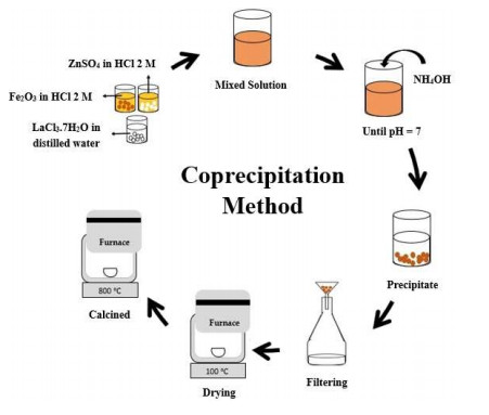
In this study, we used a natural resource, yarosite minerals, as a Fe2O3 precursor. Yarosite minerals were used for the synthesis of LaFeO3/Fe2O3 doped with ZnO via a co-precipitation method using ammonium hydroxide, which produced a light brown powder. Then, an ethanol gas sensor was prepared using a screen-printing technique and characterized using gas chamber tools at 100,200, and 300 ppm of ethanol gas to investigate the sensor's performance. Several factors that substantiate electrical properties such as crystal and morphological structures were also studied using X-Ray Diffraction (XRD) and Scanning Electron Microscopy (SEM), respectively. The crystallite size decreased from about 61.4 nm to 28.8 nm after 0.5 mol% ZnO was added. The SEM characterization images informed that the modified LaFeO3 was relatively the same but not uniform. Lastly, the sensor's electrical properties exhibited a high response of about 257% to 309% at an operating temperature that decreased from 205 ℃ to 180 ℃. This finding showed that these natural resources have the potential to be applied in the development of ethanol gas sensors in the future. Hence, yarosite minerals can be considered a good natural resource that can be further explored to produce an ethanol gas sensor with more sensitive response. In addition, this method reduces the cost of material purchase.

| [1] |
Zhang X, Lan W, Xu J, et al. (2019) ZIF-8 derived hierarchical hollow ZnO nanocages with quantum dots for sensitive ethanol gas detection. Sens Actuators B Chem 289: 144-152. https://doi.org/10.1016/j.snb.2019.03.090 doi: 10.1016/j.snb.2019.03.090

|
| [2] |
Wang C, Wang ZG, Xi R, et al. (2019) In situ synthesis of flower-like ZnO on GaN using electrodeposition and its application as ethanol gas sensor at room temperature. Sens Actuators B Chem 292: 270-276. https://doi.org/10.1016/j.snb.2019.04.140 doi: 10.1016/j.snb.2019.04.140
|
| [3] |
Zhang S, Wang C, Qu F, et al. (2019) ZnO nanoflowers modified with RuO2 for enhancing acetone sensing performance. Nanotechnology 31: 115502. https://doi.org/10.1088/1361-6528/ab5cd9 doi: 10.1088/1361-6528/ab5cd9
|
| [4] |
Wang X, Liu F, Chen X, et al. (2020) SnO2 core-shell hollow microspheres co-modification with Au and NiO nanoparticles for acetone sensing. Powder Technol 364: 159-166. https://doi.org/10.1016/j.powtec.2020.02.006 doi: 10.1016/j.powtec.2020.02.006
|
| [5] |
Yin M, Wang Y, Yu L, et al. (2020) Ag nanoparticles-modified Fe2O3@MoS2 core-shell micro/nanocomposites for high-performance NO2 gas detection at low temperature. J Alloys Compd 829: 153371. https://doi.org/10.1016/j.jallcom.2020.154471 doi: 10.1016/j.jallcom.2020.154471
|
| [6] |
Tan J, Hu J, Ren J, et al. (2020) Fast response speed of mechanically exfoliated MoS2 modified by PbS in detecting NO2. Chinese Chem Lett 31: 2103-2108. https://doi.org/10.1016/j.cclet.2020.03.060 doi: 10.1016/j.cclet.2020.03.060
|
| [7] |
Luo N, Zhang D, Xu J (2020) Enhanced CO sensing properties of Pd modified ZnO porous nanosheets. Chinese Chem Lett 31: 2033-2036. https://doi.org/10.1016/j.cclet.2020.01.002 doi: 10.1016/j.cclet.2020.01.002
|
| [8] |
Zhu K, Ma S, Tie Y, et al. (2019) Highly sensitive formaldehyde gas sensors based on Y-doped SnO2 hierarchical flower-shaped nanostructures. J Alloys Compd 792: 938-944. https://doi.org/10.1016/j.jallcom.2019.04.102 doi: 10.1016/j.jallcom.2019.04.102
|
| [9] |
Cao J, Wang S, Zhao X, et al. (2020) Facile synthesis and enhanced toluene gas sensing performances of Co3O4 hollow nanosheets. Mater Lett 263: 127215. https://doi.org/10.1016/j.matlet.2019.127215 doi: 10.1016/j.matlet.2019.127215
|
| [10] |
Zhang C, Luo Y, Xu J, et al. (2019) Room temperature conductive type metal oxide semiconductor gas sensors for NO2 detection. Sens Actuator A Phys 289: 118-133. https://doi.org/10.1016/j.sna.2019.02.027 doi: 10.1016/j.sna.2019.02.027
|
| [11] |
Liu W, Xie Y, Chen T, et al. (2019) Rationally designed mesoporous In2O3 nanofibers functionalized Pt catalyst for high-performance acetone gas sensors. Sens Actuators B Chem 298: 126871. https://doi.org/10.1016/j.snb.2019.126871 doi: 10.1016/j.snb.2019.126871
|
| [12] |
Song Z, Zhang J, Jiang J (2020) Morphological evolution, luminescence properties and a high-sensitivity ethanol gas sensor based on 3D flower-like MoS2-ZnO micro/nanosphere arrays Ceram Int 46: 6634-6640. https://doi.org/10.1016/j.ceramint.2019.11.151 doi: 10.1016/j.ceramint.2019.11.151
|
| [13] |
Zhang K, Qin S, Tang P, et al. (2020) Ultra-sensitive ethanol gas sensors based on nanosheet-assembled hierarchical ZnO-In2O3 heterostructures. J Hazard Mater 391: 122191. https://doi.org/10.1016/j.jhazmat.2020.122191 doi: 10.1016/j.jhazmat.2020.122191
|
| [14] |
Cao P, Yang Z, Navale ST, et al. (2019) Ethanol sensing behavior of Pd-nanoparticles decorated ZnO-nanorod based chemiresistive gas sensors. Sensor Actuat B Chem 298: 126850. https://doi.org/10.1016/j.snb.2019.126850 doi: 10.1016/j.snb.2019.126850
|
| [15] |
Zeng Q, Cui Y, Zhu L, et al. (2020) Increasing oxygen vacancies at room temperature in SnO2 for enhancing ethanol gas sensing. Mat Sci Semicon Proc 111: 104962. https://doi.org/10.1016/j.mssp.2020.104962 doi: 10.1016/j.mssp.2020.104962
|
| [16] |
Yu HL, Wang J, Zheng B, et al. (2020) Fabrication of single crystalline WO3 nano-belts based photoelectric gas sensor for detection of high concentration ethanol gas at room temperature. Sens Actuator A Phys 303: 111865. https://doi.org/10.1016/j.sna.2020.111865 doi: 10.1016/j.sna.2020.111865
|
| [17] |
Mao JN, Hong B, Chen HD, et al. (2020) Highly improved ethanol gas response of n-type α‑Fe2O3 bunched nanowires sensor with high-valence donor-doping. J Alloys Compd 827: 154248. https://doi.org/10.1016/j.jallcom.2020.154248 doi: 10.1016/j.jallcom.2020.154248
|
| [18] |
Cao E, Wu A, Wang H, et al. (2019) Enhanced ethanol sensing performance of Au and Cl comodified LaFeO3 nanoparticles. ACS Appl Nano Mater 2: 1541-1551. https://doi.org/10.1021/acsanm.9b00024 doi: 10.1021/acsanm.9b00024
|
| [19] |
Shingange K, Swart HC, Mhlongo, GH (2020) Design of porous p-type LaCoO3 nanofibers with remarkable response and selectivity to ethanol at low operating temperature. Sensor Actuat B Chem 308: 127670. https://doi.org/10.1016/j.snb.2020.127670 doi: 10.1016/j.snb.2020.127670
|
| [20] |
Cao E, Feng Y, Guo Z, et al. (2020) Ethanol sensing characteristics of (La, Ba)(Fe, Ti)O3 nanoparticles with impurity phases of BaTiO3 and BaCO3. J Sol‑Gel Sci Techn 96: 431-440. https://doi.org/10.1007/s10971-020-05369-x doi: 10.1007/s10971-020-05369-x
|
| [21] |
Xiang J, Chen X, Zhang X, et al. (2018) Preparation and characterization of Ba-doped LaFeO3 nanofibers by electrospinning and their ethanol sensing properties. Mater Chem Phys 213: 122-129. https://doi.org/10.1016/j.matchemphys.2018.04.024 doi: 10.1016/j.matchemphys.2018.04.024
|
| [22] | Nga PTT, My DTT, Duc NM, et al. (2021) Characteristics of porous spherical LaFeO3 as ammonia gas sensing material. Vietnam J Chem 59: 676-683. |
| [23] |
Zhang Y, Zhao J, Sun H, et al. (2018) B, N, S, Cl doped graphene quantum dots and their effect on gas-sensing properties of Ag-LaFeO3. Sensor Actuat B Chem 266: 364-374. https://doi.org/10.1016/j.snb.2018.03.109 doi: 10.1016/j.snb.2018.03.109
|
| [24] |
Zhang W, Yang B, Liu J, et al. (2017) Highly sensitive and low operating temperature SnO2 gas sensor doped by Cu and Zn two elements. Sensor Actuat B Chem 243: 982-989. https://doi.org/10.1016/j.snb.2016.12.095 doi: 10.1016/j.snb.2016.12.095
|
| [25] |
Qin J, Cui Z, Yang X, et al. (2015) Three-dimensionally ordered macroporous La1-xMgxFeO3 as high performance gas sensor to methanol. J Alloys Compd 635: 194-202. https://doi.org/10.1016/j.jallcom.2015.01.226 doi: 10.1016/j.jallcom.2015.01.226
|
| [26] |
Chen M, Wang H, Hu J, et al. (2018) Near-room-temperature ethanol gas sensor based on mesoporous Ag/Zn-LaFeO3 nanocomposite. Adv Mater Interfaces 6: 1801453. https://doi.org/10.1002/admi.201801453 doi: 10.1002/admi.201801453
|
| [27] |
Wang C, Rong Q, Zhang Y, et al. (2019) Molecular imprinting Ag-LaFeO3 spheres for highly sensitive acetone gas detection. Mater Res Bull 109: 265-272. https://doi.org/10.1016/j.materresbull.2018.09.040 doi: 10.1016/j.materresbull.2018.09.040
|
| [28] |
Koli PB, Kapadnis KH, Deshpande UG, et al. (2020) Sol-gel fabricated transition metal Cr3+, Co2+ doped lanthanum ferric oxide (LFO-LaFeO3) thin film sensors for the detection of toxic, flammable gases: A comparative study. Mat Sci Res India 17: 70-83. https://doi.org/10.13005/msri/170110 doi: 10.13005/msri/170110
|
| [29] |
Ma L, Ma SY, Qiang Z, et al. (2017) Preparation of Co-doped LaFeO3 nanofibers with enhanced acetic acid sensing properties. Mater Lett 200: 47-50. https://doi.org/10.1016/j.matlet.2017.04.096 doi: 10.1016/j.matlet.2017.04.096
|
| [30] |
Manzoor S, Husain S, Somvanshi A, et al. (2019) Impurity induced dielectric relaxor behavior in Zn doped LaFeO3. J Mater Sci Mater Electron 30: 19227-19238. https://doi.org/10.1007/s10854-019-02281-1 doi: 10.1007/s10854-019-02281-1
|
| [31] |
Tumberphale UB, Jadhav SS, Raut SD, et al. (2020) Tailoring ammonia gas sensing performance of La3+-doped copper cadmium ferrite nanostructures. Solid State Sci 100: 106089. https://doi.org/10.1016/j.solidstatesciences.2019.106089 doi: 10.1016/j.solidstatesciences.2019.106089
|
| [32] | Suhendi E, Amanda ZA, Ulhakim MT, et al. (2021) The enhancement of ethanol gas sensors response based on calcium and zinc co-doped LaFeO3/Fe2O3 thick film ceramics utilizing yarosite minerals extraction as Fe2O3 precursor. J Met Mater Miner 31: 71-77. |
| [33] |
Lai T, Fang T, Hsiao Y, et al (2019) Characteristics of Au-doped SnO2-ZnO heteronanostructures for gas sensing applications. Vacuum 166: 155-161. https://doi.org/10.1016/j.vacuum.2019.04.061 doi: 10.1016/j.vacuum.2019.04.061
|
| [34] |
Ehsani M, Hamidon MN, Toudeshki A, et al. (2016) CO2 gas sensing properties of screen-printed La2O3/SnO2 thick film. IEEE Sens J 16: 6839-6845. https://doi.org/10.1109/JSEN.2016.2587779 doi: 10.1109/JSEN.2016.2587779
|
| [35] |
Isabel RTM, Onuma S, Angkana P, et al. (2018) Printed PZT thick films implemented for functionalized gas sensors. Key Eng Mater 777: 158-162. https://doi.org/10.4028/www.scientific.net/KEM.777.158 doi: 10.4028/www.scientific.net/KEM.777.158
|
| [36] |
Moschos A, Syrovy T, Syrova L, et al. (2017) A screen-printed flexible flow sensor. Meas Sci Technol 28: 055105. https://doi.org/10.1088/1361-6501/aa5fa0 doi: 10.1088/1361-6501/aa5fa0
|
| [37] | Suhendi E, Ulhakim MT, Setiawan A, et al. (2019) The effect of SrO doping on LaFeO3 using yarosite extraction based ethanol gas sensors performance fabricated by coprecipitation method. Int J Nanoelectron Mater 12: 185-192. |
| [38] |
Kou X, Wang C, Ding M, et al. (2016) Synthesis of Co-doped SnO2 nanofibers and their enhanced gas-sensing properties. Sensor Actuat B Chem 236: 425-432. https://doi.org/10.1016/j.snb.2016.06.006 doi: 10.1016/j.snb.2016.06.006
|
| [39] |
Wang H, Wei S, Zhang F, et al. (2017) Sea urchin-like SnO2/Fe2O3 microspheres for an ethanol gas sensor with high sensitivity and fast response/recovery. J Mater Sci Mater Electron 28: 9969-9973. https://doi.org/10.1007/s10854-017-6755-3 doi: 10.1007/s10854-017-6755-3
|
| [40] |
Li Z, Yi J (2017) Enhanced ethanol sensing of Ni-doped SnO2 hollow spheres synthesized by a one-pot hydrothermal method. Sensor Actuat B Chem 243: 96-103. https://doi.org/10.1016/j.snb.2016.11.136 doi: 10.1016/j.snb.2016.11.136
|
| [41] |
Cheng Y, Guo H, Wang Y, et al. (2018) Low cost fabrication of highly sensitive ethanol sensor based on Pd-doped α-Fe2O3 porous nanotubes. Mater Res Bull 105: 21-27. https://doi.org/10.1016/j.materresbull.2018.04.025 doi: 10.1016/j.materresbull.2018.04.025
|
| [42] |
Zhang J, Liu L, Sun C, et al. (2020) Sr-doped α-Fe2O3 3D layered microflowers have high sensitivity and fast response to ethanol gas at low temperature. Chem Phys Lett 750: 137495. https://doi.org/10.1016/j.cplett.2020.137495 doi: 10.1016/j.cplett.2020.137495
|
| [43] |
Wei W, Guo S, Chen C, et al. (2017) High sensitive and fast formaldehyde gas sensor based on Ag-doped LaFeO3 nanofibers. J Alloys Compd 695: 1122-1127. https://doi.org/10.1016/j.jallcom.2016.10.238 doi: 10.1016/j.jallcom.2016.10.238
|
| [44] |
Cao E, Yang Y, Cui T, et al. (2017) Effect of synthesis route on electrical and ethanol sensing characteristics for LaFeO3-δ nanoparticles by citric sol-gel method. Appl Surf Sci 393: 134-143. https://doi.org/10.1016/j.apsusc.2016.10.013 doi: 10.1016/j.apsusc.2016.10.013
|
| [45] |
Cao E, Wang H, Wang X, et al. (2017) Enhanced ethanol sensing performance for chlorine doped nanocrystalline LaFeO3-δ powders by citric sol-gel method. Sensor Actuat B Chem 251: 885-893. https://doi.org/10.1016/j.snb.2017.05.153 doi: 10.1016/j.snb.2017.05.153
|
| [46] |
Zhang Y, Duan Z, Zou H, et al. (2018) Fabrication of electrospun LaFeO3 nanotubes via annealing technique for fast ethanol detection. Mater Lett 215: 58-61. https://doi.org/10.1016/j.matlet.2017.12.062 doi: 10.1016/j.matlet.2017.12.062
|
| [47] |
Ariyani NI, Syarif DG, Suhendi E (2017) Fabrication and characterization of thick film ceramics La0.9Ca0.1FeO3 for ethanol gas sensor using extraction of Fe2O3 from yarosite mineral. IOP Conf Ser Mater Sci Eng 384: 012037. https://doi.org/10.1088/1757-899X/384/1/012037 doi: 10.1088/1757-899X/384/1/012037
|
| [48] |
Zhou Q, Chen W, Xu L, et al. (2018) Highly sensitive carbon monoxide (CO) gas sensors based on Ni and Zn doped SnO2 nanomaterials. Ceram Int 44: 4392-4399. https://doi.org/10.1016/j.ceramint.2017.12.038 doi: 10.1016/j.ceramint.2017.12.038
|
| [49] |
Hao P, Qiu G, Song P, et al. (2020) Construction of porous LaFeO3 microspheres decorated with NiO nanosheets for high response ethanol gas sensors. Appl Surf Sci 515: 146025. https://doi.org/10.1016/j.apsusc.2020.146025 doi: 10.1016/j.apsusc.2020.146025
|
| [50] |
Srinivasan P, Ezhilan M, Kulandaisamy AJ, et al. (2019) Room temperature chemiresistive gas sensors: challenges and strategies-a mini review. J Mater Sci Mater Electron 30: 15852-15847. https://doi.org/10.1007/s10854-019-02025-1 doi: 10.1007/s10854-019-02025-1
|
| [51] |
Gao H, Wei D, Lin P, et al. (2017) The design of excellent xylene gas sensor using Sn-doped NiO hierarchical nanostructure. Sensor Actuat B Chem 253: 1152-1162. https://doi.org/10.1016/j.snb.2017.06.177 doi: 10.1016/j.snb.2017.06.177
|
| [52] |
Hu X, Zhu Z, Chen C, et al. (2017) Highly sensitive H2S gas sensors based on Pd-doped CuO nanoflowers with low operating temperature. Sensors Actuat B Chem 253: 809-817. https://doi.org/10.1016/j.snb.2017.06.183 doi: 10.1016/j.snb.2017.06.183
|
| [53] |
Singh G, Virpal, Singh RC (2019) Highly sensitive gas sensor based on Er-doped SnO2 nanostructures and its temperature dependent selectivity towards hydrogen and ethanol. Sensor Actuat B Chem 282: 373-383. https://doi.org/10.1016/j.snb.2018.11.086 doi: 10.1016/j.snb.2018.11.086
|
| [54] |
Phan TTN, Dinh TTM, Nguyen MD, et al. (2022) Hierarchically structured LaFeO3 with hollow core and porous shell as efficient sensing material for ethanol detection. Sensor Actuat B Chem 354: 131195. https://doi.org/10.1016/j.snb.2021.131195 doi: 10.1016/j.snb.2021.131195
|
| [55] |
Montazeri A, Jamali-Sheini F (2017) Enhanced ethanol gas-sensing performance of Pb-doped In2O3 nanosructures prepared by sonochemical method. Sensor Actuat B Chem 242: 778-791. https://doi.org/10.1016/j.snb.2016.09.181 doi: 10.1016/j.snb.2016.09.181
|
| [56] |
Mirzael A, Lee J, Majhi SM, et al. (2019) Resistive gas sensors based on metal-oxide nanowires. J Appl Phys 126: 241102. https://doi.org/10.1063/1.5118805 doi: 10.1063/1.5118805
|
| [57] |
Yang K, Ma J, Qiao X, et al. (2020) Hierarchical porous LaFeO3 nanostructure for efficient trace detection of formaldehyde. Sensor Actuat B Chem 313: 128022. https://doi.org/10.1016/j.snb.2020.128022 doi: 10.1016/j.snb.2020.128022
|
| [58] |
Liu C, Navale ST, Yang ZB, et al. (2017) Ethanol gas-sensing properties of hydrothermally grown α-MnO2 nanorods. J Alloys Compd 727: 362-369. https://doi.org/10.1016/j.jallcom.2017.08.150 doi: 10.1016/j.jallcom.2017.08.150
|


Figures(6) / Tables(3)

Endi Suhendi, Andini Eka Putri, Muhamad Taufik Ulhakim, Andhy Setiawan, Syarif Dani Gustaman. Investigation of ZnO doping on LaFeO3/Fe2O3 prepared from yarosite mineral extraction for ethanol gas sensor applications[J]. AIMS Materials Science, 2022, 9(1): 105-118. doi: 10.3934/matersci.2022007


 DownLoad: