This article concerns the existence of positive weak solutions of a heterogeneous elliptic boundary value problem of logistic type in a very general annulus. The novelty of this work lies in considering non-classical mixed glued boundary conditions. Namely, Dirichlet boundary conditions on a component of the boundary, and glued Dirichlet-Neumann boundary conditions on the other component of the boundary. In this paper we perform a complete analysis of the existence of positive weak solutions of the problem, giving a necessary condition on the $ \lambda $ parameter for the existence of them, and a sufficient condition for the existence of them, depending on the $ \lambda $-parameter, the spatial dimension $ N \geq 2 $ and the exponent $ q > 1 $ of the reaction term. The main technical tools used to carry out the mathematical analysis of this work are variational and monotonicity techniques. The results obtained in this paper are pioners in the field, because up the knowledge of the autor, this is the first time where this kind of logistic problems have been analyzed.
Citation: Santiago Cano-Casanova. Positive weak solutions for heterogeneous elliptic logistic BVPs with glued Dirichlet-Neumann mixed boundary conditions[J]. AIMS Mathematics, 2023, 8(6): 12606-12621. doi: 10.3934/math.2023633
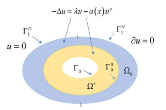
This article concerns the existence of positive weak solutions of a heterogeneous elliptic boundary value problem of logistic type in a very general annulus. The novelty of this work lies in considering non-classical mixed glued boundary conditions. Namely, Dirichlet boundary conditions on a component of the boundary, and glued Dirichlet-Neumann boundary conditions on the other component of the boundary. In this paper we perform a complete analysis of the existence of positive weak solutions of the problem, giving a necessary condition on the $ \lambda $ parameter for the existence of them, and a sufficient condition for the existence of them, depending on the $ \lambda $-parameter, the spatial dimension $ N \geq 2 $ and the exponent $ q > 1 $ of the reaction term. The main technical tools used to carry out the mathematical analysis of this work are variational and monotonicity techniques. The results obtained in this paper are pioners in the field, because up the knowledge of the autor, this is the first time where this kind of logistic problems have been analyzed.

| [1] |
H. Amann, Dual semigroups and second order linear elliptic boundary value problems, Israel J. Math., 45 (1983), 225–254. http://dx.doi.org/10.1007/BF02774019 doi: 10.1007/BF02774019

|
| [2] |
H. Amann, J. López-Gómez, A priori bounds and multiple solutions for superlinear indefinite elliptic problems, J. Differ. Equations, 146 (1998), 336–374. http://dx.doi.org/10.1006/jdeq.1998.3440 doi: 10.1006/jdeq.1998.3440
|
| [3] | H. Brézis, Análisis funcional, Madrid: Alianza Editorial, 1984. |
| [4] |
H. Brézis, L. Oswald, Remarks on sublinear elliptic equations, Nonlinear Anal.-Theor., 10 (1986), 55–64. http://dx.doi.org/10.1016/0362-546X(86)90011-8 doi: 10.1016/0362-546X(86)90011-8
|
| [5] |
S. Cano-Casanova, Principal eigenvalues of elliptic BVPs with glued Dirichlet-Robin mixed boundary conditions. Large potentials on the boundary conditions, J. Math. Anal. Appl., 491 (2020), 124364. http://dx.doi.org/10.1016/j.jmaa.2020.124364 doi: 10.1016/j.jmaa.2020.124364
|
| [6] | D. Gilbarg, N. Trudinger, Elliptic partial differential equations of second order, Berlin: Springer Verlag, 2001. http://dx.doi.org/10.1007/978-3-642-61798-0 |
| [7] |
J. Garcia-Melián, J. Sabina de Lis, J. Rossi, A bifurcation problem governed by the boundary condition I, Nonlinear Differ. Equ. Appl., 14 (2007), 499–525. http://dx.doi.org/10.1007/s00030-007-4064-x doi: 10.1007/s00030-007-4064-x
|
| [8] | M. Struwe, Variational methods, Heidelberg: Springer Verlag, 2008. http://dx.doi.org/10.1007/978-3-540-74013-1 |
Figures(1)

Santiago Cano-Casanova. Positive weak solutions for heterogeneous elliptic logistic BVPs with glued Dirichlet-Neumann mixed boundary conditions[J]. AIMS Mathematics, 2023, 8(6): 12606-12621. doi: 10.3934/math.2023633


 DownLoad: