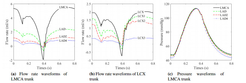
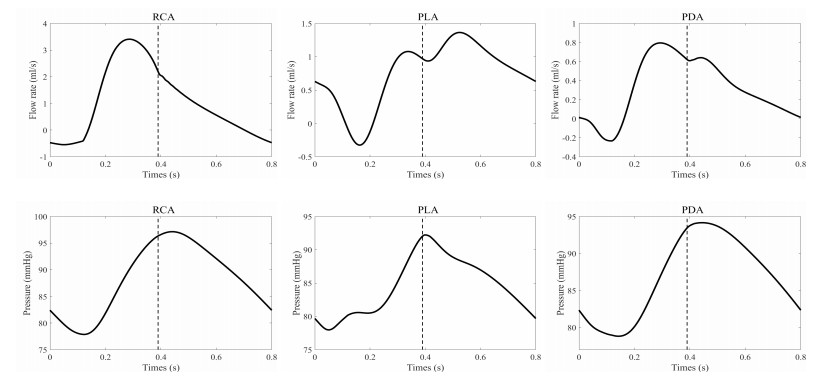
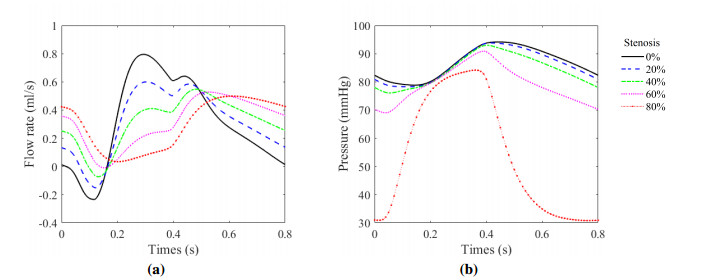
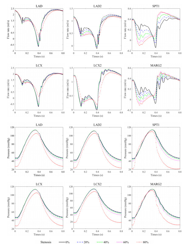
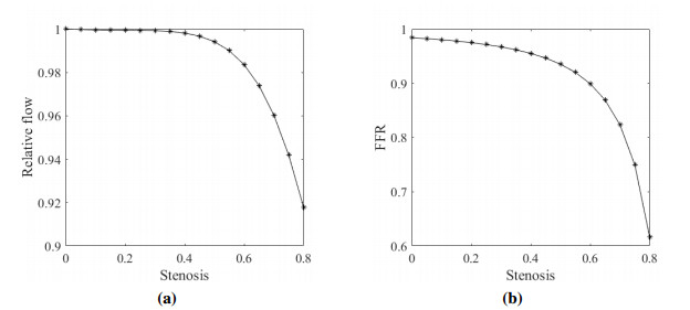
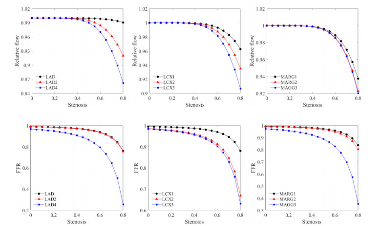
The coronary artery constitutes a vital vascular system that sustains cardiac function, with its primary role being the conveyance of indispensable nutrients to the myocardial tissue. When coronary artery disease occurs, it will affect the blood supply of the heart and induce myocardial ischemia. Therefore, it is of great significance to numerically simulate the coronary artery and evaluate its blood supply capacity. In this article, the coronary artery lumped parameter model was derived based on the relationship between circuit system parameters and cardiovascular system parameters, and the blood supply capacity of the coronary artery in healthy and stenosis states was studied. The aortic root pressure calculated by the aortic valve fluid-structure interaction (AV FSI) simulator was employed as the inlet boundary condition. To emulate the physiological phenomenon of sudden pressure drops resulting from an abrupt reduction in blood vessel radius, a head loss model was connected at the coronary artery's entrance. For each coronary artery outlet, the symmetric structured tree model was appended to simulate the terminal impedance of the missing downstream coronary arteries. The particle swarm optimization (PSO) algorithm was used to optimize the blood flow viscous resistance, blood flow inertia, and vascular compliance of the coronary artery model. In the stenosis states, the relative flow and fractional flow reserve (FFR) calculated by numerical simulation corresponded to the published literature data. It was anticipated that the proposed model can be readily adapted for clinical application, serving as a valuable reference for diagnosing and treating patients.
Citation: Li Cai, Qian Zhong, Juan Xu, Yuan Huang, Hao Gao. A lumped parameter model for evaluating coronary artery blood supply capacity[J]. Mathematical Biosciences and Engineering, 2024, 21(4): 5838-5862. doi: 10.3934/mbe.2024258
The coronary artery constitutes a vital vascular system that sustains cardiac function, with its primary role being the conveyance of indispensable nutrients to the myocardial tissue. When coronary artery disease occurs, it will affect the blood supply of the heart and induce myocardial ischemia. Therefore, it is of great significance to numerically simulate the coronary artery and evaluate its blood supply capacity. In this article, the coronary artery lumped parameter model was derived based on the relationship between circuit system parameters and cardiovascular system parameters, and the blood supply capacity of the coronary artery in healthy and stenosis states was studied. The aortic root pressure calculated by the aortic valve fluid-structure interaction (AV FSI) simulator was employed as the inlet boundary condition. To emulate the physiological phenomenon of sudden pressure drops resulting from an abrupt reduction in blood vessel radius, a head loss model was connected at the coronary artery's entrance. For each coronary artery outlet, the symmetric structured tree model was appended to simulate the terminal impedance of the missing downstream coronary arteries. The particle swarm optimization (PSO) algorithm was used to optimize the blood flow viscous resistance, blood flow inertia, and vascular compliance of the coronary artery model. In the stenosis states, the relative flow and fractional flow reserve (FFR) calculated by numerical simulation corresponded to the published literature data. It was anticipated that the proposed model can be readily adapted for clinical application, serving as a valuable reference for diagnosing and treating patients.

| [1] |
C. W. Tsao, A. W. Aday, Z. I. Almarzooq, A. Alonso, A. Z. Beaton, M. S. Bittencourt, et al., Heart disease and stroke statistics–2022 update: A report from the american heart association, Circulation, 145 (2022), e153–e639. https://doi.org/10.1161/CIR.0000000000001052 doi: 10.1161/CIR.0000000000001052

|
| [2] |
L. Papamanolis, H. J. Kim, C. Jaquet, M. Sinclair, M. Schaap, I. Danad, et al., Myocardial perfusion simulation for coronary artery disease: A coupled patient-specific multiscale model, Ann. Biomed. Eng., 49 (2021), 1432–1447. https://doi.org/10.1007/s10439-020-02681-z doi: 10.1007/s10439-020-02681-z
|
| [3] |
V. C. Rideout, J. A. Katra, Computer simulation study of the pulmonary circulation, Simulation, 12 (1969), 239–245. https://doi.org/10.1177/003754976901200505 doi: 10.1177/003754976901200505
|
| [4] |
M. F. Snyder, V. C. Rideout, Computer simulation studies of the venous circulation, IEEE Trans. Biomed. Eng., BME-16 (1969), 325–334. https://doi.org/10.1109/TBME.1969.4502663 doi: 10.1109/TBME.1969.4502663
|
| [5] |
V. C. Rideout, Cardiovascular system simulation in biomedical engineering education, IEEE Trans. Biomed. Eng., BME-19 (1972), 101–107. https://doi.org/10.1109/TBME.1972.324103 doi: 10.1109/TBME.1972.324103
|
| [6] |
F. Liang, H. Liu, A closed-loop lumped parameter computational model for human cardiovascular system, JSME Int. J., Ser. C, 48 (2005), 484–493. https://doi.org/10.1299/jsmec.48.484 doi: 10.1299/jsmec.48.484
|
| [7] |
J. Wang, B. Tie, W. Welkowitz, J. Kostis, J. Semmlow, Incremental network analogue model of the coronary artery, Med. Biol. Eng. Comput., 27 (1989), 416–422. https://doi.org/10.1007/BF02441434 doi: 10.1007/BF02441434
|
| [8] |
S. Mantero, R. Pietrabissa, R. Fumero, The coronary bed and its role in the cardiovascular system: A review and an introductory single-branch model, J. Biomed. Eng., 14 (1992), 109–116. https://doi.org/10.1016/0141-5425(92)90015-d doi: 10.1016/0141-5425(92)90015-d
|
| [9] |
R. Pietrabissa, S. Mantero, T. Marotta, L. Menicanti, A lumped parameter model to evaluate the fluid dynamics of different coronary bypasses, Med. Eng. Phys., 18 (1996), 477–484. https://doi.org/10.1016/1350-4533(96)00002-1 doi: 10.1016/1350-4533(96)00002-1
|
| [10] |
Z. Duanmu, M. Yin, X. Fan, X. Yang, X. Luo, A patient-specific lumped-parameter model of coronary circulation, Sci. Rep., 8 (2018), 874. https://doi.org/10.1038/s41598-018-19164-w doi: 10.1038/s41598-018-19164-w
|
| [11] |
N. Westerhof, G. Elzinga, P. Sipkema, An artificial arterial system for pumping hearts, J. Appl. Physiol., 31 (1971), 776–781. https://doi.org/10.1152/jappl.1971.31.5.776 doi: 10.1152/jappl.1971.31.5.776
|
| [12] | A. S. Olufsen, Modeling the Arterial System with Reference to an Anesthesia Simulator, PhD. thesis, Roskilde University, 1998. |
| [13] |
M. S. Olufsen, Structured tree outflow condition for blood flow in larger systemic arteries, J. Appl. Physiol. Heart Circulat. Physiol., 276 (1999), H257–H268. https://doi.org/10.1152/ajpheart.1999.276.1.H257 doi: 10.1152/ajpheart.1999.276.1.H257
|
| [14] |
M. S. Olufsen, C. S. Peskin, W. Y. Kim, E. M. Pedersen, A. Nadim, J. Larsen, Numerical simulation and experimental validation of blood flow in arteries with structured-tree outflow conditions, Ann. Biomed. Eng., 28 (2000), 1281–1299. https://doi.org/10.1114/1.1326031 doi: 10.1114/1.1326031
|
| [15] |
Y. Zhang, T. Furusawa, S. F. Sia, M. Umezu, Y. Qian, Proposition of an outflow boundary approach for carotid artery stenosis CFD simulation, Comput. Method Biomech. Biomed. Eng., 16 (2013), 488–494. https://doi.org/10.1080/10255842.2011.625358 doi: 10.1080/10255842.2011.625358
|
| [16] |
C. Pagiatakis, J. C. Tardif, P. L. L'Allier, R. Mongrain, A numerical investigation of the functionality of coronary bifurcation lesions with respect to lesion configuration and stenosis severity, J. Biomech., 48 (2015), 3103–3111. https://doi.org/10.1016/j.jbiomech.2015.07.018 doi: 10.1016/j.jbiomech.2015.07.018
|
| [17] |
C. Pagiatakis, J. C. Tardif, P. L. L'Allier, R. Mongrain, Effect of stenosis eccentricity on the functionality of coronary bifurcation lesions—A numerical study, Med. Biol. Eng. Comput., 55 (2017), 2079–2095. https://doi.org/10.1007/s11517-017-1653-7 doi: 10.1007/s11517-017-1653-7
|
| [18] |
A. S. Yong, A. C. Ng, D. Brieger, H. C. Lowe, M. K. Ng, L. Kritharides, Three-dimensional and two-dimensional quantitative coronary angiography, and their prediction of reduced fractional flow reserve, Eur. Heart J., 32 (2011), 345–353. https://doi.org/10.1093/eurheartj/ehq259 doi: 10.1093/eurheartj/ehq259
|
| [19] |
S. Sen, J. Escaned, I. S. Malik, G. W. Mikhail, R. A. Foale, R. Mila, et al., Development and validation of a new adenosine-independent index of stenosis severity from coronary wave-intensity analysis: results of the advise (adenosine vasodilator independent stenosis evaluation) study, J. Am. Coll. Cardiol., 59 (2012), 1392–1402. https://doi.org/10.1016/j.jacc.2011.11.003 doi: 10.1016/j.jacc.2011.11.003
|
| [20] |
Z. Yan, Z. Yao, W. Guo, D. Shang, R. Chen, J. Liu, et al., Impact of pressure wire on fractional flow reserve and hemodynamics of the coronary arteries: A computational and clinical study, IEEE Trans. Biomed. Eng., 70 (2022), 1683–1691. https://doi.org/10.1109/tbme.2022.3225188 doi: 10.1109/tbme.2022.3225188
|
| [21] |
B. De Bruyne, J. Bartunek, S. U. Sys, G. R. Heyndrickx, Relation between myocardial fractional flow reserve calculated from coronary pressure measurements and exercise-induced myocardial ischemia, Circulation, 92 (1995), 39–46. https://doi.org/10.1161/01.cir.92.1.39 doi: 10.1161/01.cir.92.1.39
|
| [22] |
N. H. Pijls, B. Van Gelder, P. Van der Voort, K. Peels, F. A. Bracke, H. J. Bonnier, et al., Fractional flow reserve: A useful index to evaluate the influence of an epicardial coronary stenosis on myocardial blood flow, Circulation, 92 (1995), 3183–3193. https://doi.org/10.1161/01.cir.92.11.3183 doi: 10.1161/01.cir.92.11.3183
|
| [23] |
L. Cai, R. Zhang, Y. Li, G. Zhu, X. Ma, Y. Wang, et al., The comparison of different constitutive laws and fiber architectures for the aortic valve on fluid-structure interaction simulation, Front. Physiol., 12 (2021), 725. https://doi.org/10.3389/fphys.2021.682893 doi: 10.3389/fphys.2021.682893
|
| [24] |
L. Cai, Y. Hao, P. Ma, G. Zhu, X. Luo, H. Gao, Fluid-structure interaction simulation of calcified aortic valve stenosis, Math. Biosci. Eng., 19 (2022), 13172–13192. https://doi.org/10.3934/mbe.2022616 doi: 10.3934/mbe.2022616
|
| [25] |
N. Westerhof, J. W. Lankhaar, B. E. Westerhof, The arterial windkessel, Med. Biol. Eng. Comput., 47 (2009), 131–141. https://doi.org/10.1007/s11517-008-0359-2 doi: 10.1007/s11517-008-0359-2
|
| [26] |
Q. Wang, W. Sun, Finite element modeling of mitral valve dynamic deformation using patient-specific multi-slices computed tomography scans, Ann. Biomed. Eng., 41 (2013), 142–153. https://doi.org/10.1007/s10439-012-0620-6 doi: 10.1007/s10439-012-0620-6
|
| [27] |
N. Stergiopulos, B. E. Westerhof, N. Westerhof, Total arterial inertance as the fourth element of the windkessel model, J. Appl. Physiol. Heart Circulat. Physiol., 276 (1999), H81–H88. https://doi.org/10.1152/ajpheart.1999.276.1.H81 doi: 10.1152/ajpheart.1999.276.1.H81
|
| [28] |
B. E. Griffith, Immersed boundary model of aortic heart valve dynamics with physiological driving and loading conditions, Int. J. Numer. Method. Biomed. Eng., 28 (2012), 317–345. https://doi.org/10.1002/cnm.1445 doi: 10.1002/cnm.1445
|
| [29] |
B. E. Griffith, X. Luo, Hybrid finite difference/finite element immersed boundary method, Int. J. Numer. Method. Biomed. Eng., 33 (2017), e2888. https://doi.org/10.1002/cnm.2888 doi: 10.1002/cnm.2888
|
| [30] |
H. Gao, X. Ma, N. Qi, C. Berry, B. E. Griffith, X. Luo, A finite strain nonlinear human mitral valve model with fluid-structure interaction, Int. J. Numer. Method. Biomed. Eng., 30 (2014), 1597–1613. https://doi.org/10.1002/cnm.2691 doi: 10.1002/cnm.2691
|
| [31] |
C. S. Peskin, The immersed boundary method, Acta Numer., 11 (2002), 479–517. https://doi.org/10.1016/j.jcp.2023.112148 doi: 10.1016/j.jcp.2023.112148
|
| [32] |
D. Boffi, L. Gastaldi, L. Heltai, C. S. Peskin, On the hyper-elastic formulation of the immersed boundary method, Comput. Methods Appl. Mech. Eng., 197 (2008), 2210–2231. https://doi.org/10.1016/j.cma.2007.09.015 doi: 10.1016/j.cma.2007.09.015
|
| [33] | C. Vlachopoulos, M. O'Rourke, W. W. Nichols, McDonald's Blood Flow in Arteries: Theoretical, Experimental and Clinical Principles, 6th edition, CRC Press, London, 2012. https://doi.org/10.1201/b13568 |
| [34] |
Y. Liu, L. Cai, Y. Chen, P. Ma, Q. Zhong, Variable separated physics-informed neural networks based on adaptive weighted loss functions for blood flow model, Comput. Math. Appl., 153 (2024), 108–122. https://doi.org/10.1016/j.camwa.2023.11.018 doi: 10.1016/j.camwa.2023.11.018
|
| [35] | L. R. Waite, Biofluid Mechanics in Cardiovascular Systems, McGraw Hill Professional, 2005. https://doi.org/10.1036/0071447881 |
| [36] |
J. R. Mitchell, J. J. Wang, Expanding application of the Wiggers diagram to teach cardiovascular physiology, Adv. Physiol. Educ., 38 (2014), 170–175. https://doi.org/10.1152/advan.00123.2013 doi: 10.1152/advan.00123.2013
|
| [37] |
V. Fester, B. Mbiya, P. Slatter, Energy losses of non-Newtonian fluids in sudden pipe contractions, Chem. Eng. J., 145 (2008), 57–63. https://doi.org/10.1016/j.cej.2008.03.003 doi: 10.1016/j.cej.2008.03.003
|
| [38] |
A. Iberall, Anatomy and steady flow characteristics of the arterial system with an introduction to its pulsatile characteristics, Math. Biosci., 1 (1967), 375–395. https://doi.org/10.1016/0025-5564(67)90009-0 doi: 10.1016/0025-5564(67)90009-0
|
| [39] |
H. J. Kim, I. Vignon-Clementel, J. Coogan, C. Figueroa, K. Jansen, C. Taylor, Patient-specific modeling of blood flow and pressure in human coronary arteries, Ann. Biomed. Eng., 38 (2010), 3195–3209. https://doi.org/10.1007/s10439-010-0083-6 doi: 10.1007/s10439-010-0083-6
|
| [40] | L. P. Huelsman, Basic Circuit Theory: with Digital Computations, Prentice-Hall, 1972. |
| [41] |
B. S. Gow, D. Schonfeld, D. J. Patel, The dynamic elastic properties of the canine left circumflex coronary artery, J. Biomech., 7 (1974), 389–395. https://doi.org/10.1016/0021-9290(74)90001-3 doi: 10.1016/0021-9290(74)90001-3
|
| [42] |
W. Welkowitz, Engineering hemodynamics: Application to cardiac assist devices, J. Clin. Eng., 13 (1988), 79. https://doi.org/10.1097/00004669-198803000-00003 doi: 10.1097/00004669-198803000-00003
|
| [43] | P. Siena, M. Girfoglio, G. Rozza, Fast and accurate numerical simulations for the study of coronary artery bypass grafts by artificial neural networks, in Reduced Order Models for the Biomechanics of Living Organs, (2023), 167–183. |
| [44] |
N. M. Marazzi, G. Guidoboni, M. Zaid, L. Sala, S. Ahmad, L. Despins, et al., Combining physiology-based modeling and evolutionary algorithms for personalized, noninvasive cardiovascular assessment based on electrocardiography and ballistocardiography, Front. Physiol., 12 (2022), 739035. https://doi.org/10.3389/fphys.2021.739035 doi: 10.3389/fphys.2021.739035
|
| [45] | J. Kennedy, R. Eberhart, Particle swarm optimization, in International Conference on Neural Networks, 4 (1995), 1942–1948. https://doi.org/10.1109/ICNN.1995.488968 |
| [46] | Y. Shi, R. Eberhart, A modified particle swarm optimizer, in IEEE International Conference on Evolutionary Computation, (1998), 69–73. https://doi.org/10.1109/ICEC.1998.699146 |
| [47] |
J. R. Womersley, Oscillatory flow in arteries: The constrained elastic tube as a model of arterial flow and pulse transmission, Phys. Med. Biol., 2 (1957), 178–187. https://doi.org/10.1088/0031-9155/2/2/305 doi: 10.1088/0031-9155/2/2/305
|
| [48] |
N. H. Pijls, B. De Bruyne, Coronary pressure measurement and fractional flow reserve, Heart, 80 (1998), 539–542. https://doi.org/10.1136/hrt.80.6.539 doi: 10.1136/hrt.80.6.539
|
| [49] |
J. H. Lee, A. D. Rygg, E. M. Kolahdouz, S. Rossi, S. M. Retta, N. Duraiswamy, et al., Fluid-structure interaction models of bioprosthetic heart valve dynamics in an experimental pulse duplicator, Ann. Biomed. Eng., 48 (2020), 1475–1490. https://doi.org/10.1007/s10439-020-02466-4 doi: 10.1007/s10439-020-02466-4
|
| [50] |
G. Zhu, M. B. Ismail, M. Nakao, Q. Yuan, J. H. Yeo, Numerical and in-vitro experimental assessment of the performance of a novel designed expanded-polytetrafluoroethylene stentless bi-leaflet valve for aortic valve replacement, PLoS One, 14 (2019), e0210780. https://doi.org/10.1371/journal.pone.0210780 doi: 10.1371/journal.pone.0210780
|
| [51] |
L. H. Opie, Heart physiology: from cell to circulation, Circulation, 110 (2004), e313. https://doi.org/10.1161/01.cir.0000143724.99618.62 doi: 10.1161/01.cir.0000143724.99618.62
|
| [52] |
Y. Huo, G. S. Kassab, A hybrid one-dimensional/womersley model of pulsatile blood flow in the entire coronary arterial tree, J. Appl. Physiol. Heart Circulat. Physiol., 292 (2007), H2623–H2633. https://doi.org/10.1152/ajpheart.00987.2006 doi: 10.1152/ajpheart.00987.2006
|
| [53] |
P. Meimoun, S. Sayah, A. Luycx-Bore, J. Boulanger, F. Elmkies, T. Benali, et al., Comparison bween non-invasive coronary flow reserve and fractional flow reserve to assess the functional significance of left anterior descending artery stenosis of intermediate severity, J. Am. Soc. Echocardiog., 24 (2011), 374–381. https://doi.org/10.1016/j.echo.2010.12.007 doi: 10.1016/j.echo.2010.12.007
|
| [54] |
M. Hamilos, O. Muller, T. Cuisset, A. Ntalianis, G. Chlouverakis, G. Sarno, et al., Long-term clinical outcome after fractional flow reserve-guided treatment in patients with angiographically equivocal left main coronary artery stenosis, Circulation, 120 (2009), 1505–1512. https://doi.org/10.1161/circulationaha.109.850073 doi: 10.1161/circulationaha.109.850073
|
| [55] |
B. K. Koo, K. W. Park, H. J. Kang, Y. S. Cho, W. Y. Chung, T. J. Youn, et al., Physiological evaluation of the provisional side-branch intervention strategy for bifurcation lesions using fractional flow reserve, Eur. Heart J., 29 (2008), 726–732. https://doi.org/10.1093/eurheartj/ehn045 doi: 10.1093/eurheartj/ehn045
|
| [56] |
N. Pijls, J. Van Son, R. L. Kirkeeide, B. De Bruyne, K. L. Gould, Experimental basis of determining maximum coronary, myocardial, and collateral blood flow by pressure measurements for assessing functional stenosis severity before and after percutaneous transluminal coronary angioplasty, Circulation, 87 (1993), 1354–1367. https://doi.org/10.1161/01.cir.87.4.1354 doi: 10.1161/01.cir.87.4.1354
|
| [57] |
N. H. Pijls, J. W. E. Sels, Functional measurement of coronary stenosis, J. Am. Coll. Cardiol., 59 (2012), 1045–1057. https://doi.org/10.1016/j.jacc.2011.09.077 doi: 10.1016/j.jacc.2011.09.077
|
| [58] |
M. P. Opolski, C. Kepka, S. Achenbach, J. Pregowski, M. Kruk, A. D. Staruch, et al., Advanced computed tomographic anatomical and morphometric plaque analysis for prediction of fractional flow reserve in intermediate coronary lesions, Eur. J. Radiol., 83 (2014), 135–141. https://doi.org/10.1016/j.ejrad.2013.10.005 doi: 10.1016/j.ejrad.2013.10.005
|
Figures(14) / Tables(2)

Li Cai, Qian Zhong, Juan Xu, Yuan Huang, Hao Gao. A lumped parameter model for evaluating coronary artery blood supply capacity[J]. Mathematical Biosciences and Engineering, 2024, 21(4): 5838-5862. doi: 10.3934/mbe.2024258


 DownLoad: