Branch flow distribution approach and its application in the calculation of fractional flow reserve in stenotic coronary artery

Honghui Zhang; Jun Xia; Yinlong Yang; Qingqing Yang; Hongfang Song; Jinjie Xie; Yue Ma; Yang Hou; Aike Qiao; Honghui Zhang; Jun Xia; Yinlong Yang; Qingqing Yang; Hongfang Song; Jinjie Xie; Yue Ma; Yang Hou; Aike Qiao

doi:10.3934/mbe.2021299

Mathematical Biosciences and Engineering

2021, Volume 18, Issue 5: 5978-5994. doi: 10.3934/mbe.2021299

Previous Article Next Article

Research article Special Issues

Branch flow distribution approach and its application in the calculation of fractional flow reserve in stenotic coronary artery

1.
Faculty of Environment and Life, Beijing University of Technology, Beijing 100124, China
2.
Intelligent Physiological Measurement and Clinical Translation, Beijing International Base for Scientific and Technological Cooperation, Beijing 100124, China
3.
School of Biomedical Engineering, Beijing Key Laboratory of Fundamental Research on Biomechanics in Clinical Application, Capital Medical University, Beijing 100069, China
4.
Beijing Anzhen Hospital, Capital Medical University, Beijing 100029, China
5.
Shengjing Hospital, China Medical University, Shenyang 110001, China

Received: 15 April 2021 Accepted: 23 June 2021 Published: 02 July 2021

Objective
To calculate fractional flow reserve (FFR) based on computed tomography angiography (i.e., FFR_CT) by considering the branch flow distribution in the coronary arteries.

Background
FFR is the gold standard to diagnose myocardial ischemia caused by coronary stenosis. An accurate and noninvasive method for obtaining total coronary blood flow is needed for the calculation of FFR_CT.

Methods
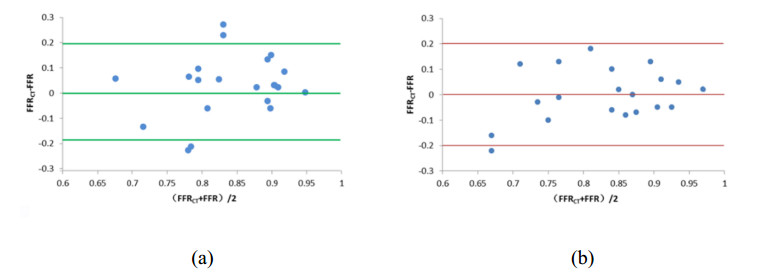
A mathematical model for estimating the coronary blood flow rate and two approaches for setting the patient-specific flow boundary condition were proposed. Coronary branch flow distribution methods based on a volume-flow approach and a diameter-flow approach were employed for the numerical simulation of FFR_CT. The values of simulated FFR_CT for 16 patients were compared with their clinically measured FFR.

Results
The ratio of total coronary blood flow to cardiac output and the myocardial blood flow under the condition of hyperemia were 16.97% and 4.07 mL/min/g, respectively. The errors of FFR_CT compared with clinical data under the volume-flow approach and diameter-flow approach were 10.47% and 11.76%, respectively, the diagnostic accuracies of FFR_CT were 65% and 85%, and the consistencies were 95% and 90%.

Conclusions
The mathematical model for estimating the coronary blood flow rate and the coronary branch flow distribution method can be applied to calculate the value of clinical noninvasive FFR_CT.
- coronary artery disease,
- hemodynamics,
- endovascular intervention,
- catheterization,
- diagnosis
Citation: Honghui Zhang, Jun Xia, Yinlong Yang, Qingqing Yang, Hongfang Song, Jinjie Xie, Yue Ma, Yang Hou, Aike Qiao. Branch flow distribution approach and its application in the calculation of fractional flow reserve in stenotic coronary artery[J]. Mathematical Biosciences and Engineering, 2021, 18(5): 5978-5994. doi: 10.3934/mbe.2021299

Related Papers:

Abstract

Objective

To calculate fractional flow reserve (FFR) based on computed tomography angiography (i.e., FFR_CT) by considering the branch flow distribution in the coronary arteries.

Background

FFR is the gold standard to diagnose myocardial ischemia caused by coronary stenosis. An accurate and noninvasive method for obtaining total coronary blood flow is needed for the calculation of FFR_CT.

Methods

A mathematical model for estimating the coronary blood flow rate and two approaches for setting the patient-specific flow boundary condition were proposed. Coronary branch flow distribution methods based on a volume-flow approach and a diameter-flow approach were employed for the numerical simulation of FFR_CT. The values of simulated FFR_CT for 16 patients were compared with their clinically measured FFR.

Results

The ratio of total coronary blood flow to cardiac output and the myocardial blood flow under the condition of hyperemia were 16.97% and 4.07 mL/min/g, respectively. The errors of FFR_CT compared with clinical data under the volume-flow approach and diameter-flow approach were 10.47% and 11.76%, respectively, the diagnostic accuracies of FFR_CT were 65% and 85%, and the consistencies were 95% and 90%.

Conclusions

The mathematical model for estimating the coronary blood flow rate and the coronary branch flow distribution method can be applied to calculate the value of clinical noninvasive FFR_CT.

References

[1]	E. Conte, J. Sonck, S. Mushtaq, C. Collet, T. Mizukami, E. Barbato, et al., FFR_CT and CT perfusion: A review on the evaluation of functional impact of coronary artery stenosis by cardiac CT, Int. J. Cardiol., 9 (2020), 289-296.
[2]	A. Cesaro, F. Gragnano, D. D. Girolamo, E. Moscarella, V. Diana, I. Pariggiano, et al., Functional assessment of coronary stenosis: an overview of available techniques. Is quantitative flow ratio a step to the future?, Expert. Rev. Cardiovasc. Ther., 16 (2018), 951-962. doi: 10.1080/14779072.2018.1540303
[3]	G. Y. Li, H. R. Wang, M. Z. Zhang, S. Tupin, A. K. Qiao, Y. J. Liu, et al., Prediction of 3D cardiovascular hemodynamics before and after coronary artery bypass surgery via deep learning, Commun. Biol., 99 (2021), 1-12.
[4]	N. S. Kleiman, Bringing it all together: integration of physiology with anatomy during cardiac catheterization, J. Am. Coll. Cardiol., 58 (2011), 1219-1221. doi: 10.1016/j.jacc.2011.06.019
[5]	C. A. Taylor, T. A. Fonte, J. K. Min, Computational fluid dynamics applied to cardiac computed tomography for noninvasive quantification of fractional flow reserve: scientific basis, J. Am. Coll. Cardiol., 61 (2013), 2233-2241. doi: 10.1016/j.jacc.2012.11.083
[6]	J. K. Min, C. A. Taylor, S. Achenbach, B. K. Koo, J. Leipsic, B. L. Nørgaard, et al., Noninvasive fractional flow reserve derived from coronary CT angiography: clinical data and scientific principles, JACC Cardiovasc. Imaging, 8 (2015), 1209-1222. doi: 10.1016/j.jcmg.2015.08.006
[7]	C. Tesche, C. N. D. Cecco, M. H. Albrecht, T. M. Duguay, R. R. Bayer, S. E. Litwin, et al., Coronary CT angiography-derived fractional flow reserve, Radiology, 285 (2017), 17-33. doi: 10.1148/radiol.2017162641
[8]	M. van Assen, C. N. D. Cecco, M. Eid, P. von Knebel Doeberitz, M. Scarabello, F. Lavra, et al., Prognostic value of CT myocardial perfusion imaging and CT-derived fractional flow reserve for major adverse cardiac events in patients with coronary artery disease, J. Cardiovasc. Comput. Tomogr., 13 (2019), 26-33. doi: 10.1016/j.jcct.2019.02.005
[9]	K. Nieman. The feasibility, findings and future of CT-FFR in the emergency ward, J. Cardiovasc. Comput. Tomogr., 19 (2019), 287-288.
[10]	B. K. Koo, A. Erglis, J. H. Doh, D. V. Daniels, S. Jegere, H. S. Kim, et al., Diagnosis of ischemia-causing coronary stenoses by noninvasive fractional flow reserve computed from coronary computed tomographic angiograms. Results from the prospective multicenter DISCOVER-FLOW (diagnosis of ischemia-causing stenoses obtained via noninvasive fractional flow reserve) study, J. Am. Coll. Cardiol., 58 (2011), 1989-1997. doi: 10.1016/j.jacc.2011.06.066
[11]	J. K. Min, B. K. Koo, A. Erglis, J. H. Doh, D. V. Daniels, S. Jegere, et al., Effect of image quality on diagnostic accuracy of noninvasive fractional flow reserve: results from the prospective multicenter international DISCOVER-FLOW study, J. Cardiovasc. Comput. Tomogr., 6 (2012), 191-199. doi: 10.1016/j.jcct.2012.04.010
[12]	J. K. Min, D. S. Berman, M. J. Budoff, F. A. Jaffer, J. Leipsic, M. B. Leon MB, et al., Rationale and design of the DeFACTO (determination of fractional flow reserve by anatomic computed tomographic angiography) study, J. Cardiovasc. Comput. Tomogr., 5 (2011), 301-309. doi: 10.1016/j.jcct.2011.08.003
[13]	J. K. Min, J. Leipsic, M. J. Pencina, D. S. Berman, B. K. Koo, C. van Mieghem, et al., Diagnostic accuracy of fractional flow reserve from anatomic CT angiography, JAMA, 308 (2012), 1237-1245. doi: 10.1001/2012.jama.11274
[14]	R Nakazato, H. B. Park, D. S. Berman, H. Gransar, B. K. Koo, A. Erglis, et al., Noninvasive fractional flow reserve derived from computed tomography angiography for coronary lesions of intermediate stenosis severity results from the DeFACTO study, Circ. Cardiovasc. Imaging, 6 (2013), 881-889. doi: 10.1161/CIRCIMAGING.113.000297
[15]	J. Leipsic, T. H. Yang, A. Thompson, B. K. Koo, G. B. J. Mancini, C. Taylor, et al., CT angiography (CTA) and diagnostic performance of noninvasive fractional flow reserve: results from the determination of fractional flow reserve by anatomic CTA (DEFACTO) study, AJR. Am. J. Roentgenol., 202 (2014), 989-994. doi: 10.2214/AJR.13.11441
[16]	S. Gaur, S. Achenbach, L. Leipsic, L. Mauri, H. G. Bezerra, Jensen JM, et al., Rationale and design of the HeartFlowNXT (heartflow analysis of coronary blood flow using CT angiography: next steps) study, J. Cardiovasc. Comput. Tomogr., 7(2013), 279-288. doi: 10.1016/j.jcct.2013.09.003
[17]	B. L. Nørgaard, J. Leipsic, S. Gaur, S. Seneviratne, B. S. Ko, H. Ito, et al., Diagnostic performance of noninvasive fractional flow reserve derived from coronary computed tomography angiography in suspected coronary artery disease: The NXT trial (analysis of coronary blood flow using CT angiography: next steps), J. Am. Coll. Cardiol., 63 (2014), 1145-1155. doi: 10.1016/j.jacc.2013.11.043
[18]	T. Miyoshi, K. Osawa, H. Ito, S. Kanazawa, T. Kimura, H, Shiomi, et al., Non-invasive computed fractional flow reserve from computed tomography (CT) for diagnosing coronary artery disease, Circ. J., 79 (2015), 406-412. doi: 10.1253/circj.CJ-14-1051
[19]	K. Tanaka, H. G. Bezerra, S. Gaur, G. F. Attizzani, H. E. Bøtker, M. A. Costa, et al., Comparison between nNon-invasive (coronary computed tomography angiography derived) and invasive-fractional flow reserve in patients with serial stenoses within one coronary artery-A NXT trial substudy, Ann. Biomed. Eng., 44 (2016), 580-589. doi: 10.1007/s10439-015-1436-y
[20]	C. X. Tang, C. Y. Liu, M. J. Lu, U. J. Schoepf, C. Tesche, R. R. Bayer, et al., CT FFR for ischemia-specific CAD with a new computational fluid dynamics algorithm: a Chinese multicenter study, JACC Cardiovasc. Imaging, 13 (2020), 980-990. doi: 10.1016/j.jcmg.2019.06.018
[21]	L. D. Rasmussen, S. Winther, J. Westra, C. Isaksen, J. A. Ejlersen, L. Brix, et al., Danish study of non-Invasive testing in coronary artery disease 2 (Dan-NICAD 2): Study design for a controlled study of diagnostic accuracy, Am. Heart. J, 215 (2019), 114-128. doi: 10.1016/j.ahj.2019.03.016
[22]	J. M. Carson, S. Pant, C. Roobottom, R. Alcock, Non-invasive coronary CT angiography-derived fractional flow reserve: A benchmark study comparing the diagnostic performance of four different computational methodologies, Int. J. Numer. Method. Biomed. Eng., 17 (2019), e3235.
[23]	J. S. Choy, G. S. Kassab. Scaling of myocardial mass to flow and morphometry of coronary arteries, J. Appl. Physiol., 104 (2008), 1281-1286. doi: 10.1152/japplphysiol.01261.2007
[24]	C. J. Arthurs, K. D. Lau, K. N. Asrress, S. R. Redwood, C. A. Figueroa, A mathematical model of coronary blood flow control: simulation of patient-specific three-dimensional hemodynamics during exercise, Am. J. Physiol. Heart Circ. Physiol., 310 (2016), 1242-1258. doi: 10.1152/ajpheart.00517.2015
[25]	Z. Duanmu, W. W. Chen, H. Gao, X. L. Yang, X. Luo, N. A. Hill, A one-dimensional hemodynamic model of the coronary arterial tree, Front. Physiol., 10 (2019), 853.
[26]	Z. Duanmu, M. Yin, X. Fan, X. Yang, X. Luo, A patient-specific lumped-parameter model of coronary circulation, Sci. Rep., 8 (2018), 1-10.
[27]	Y. Huo, G. S. Kassab, The scaling of blood flow resistance: from a single vessel to the entire distal tree, Biophys. J., 96 (2009), 339-346. doi: 10.1016/j.bpj.2008.09.038
[28]	J. M. Zhang, L. Zhong, T. Luo, A. M. Lomarda, Y. Huo, J. Yap, et al., Simplified models of non-invasive fractional flow reserve based on CT images, PLoS One, 11 (2016), e0153070. doi: 10.1371/journal.pone.0153070
[29]	M. Abe, H. Tomiyama, H. Yoshida, D. Doba, Diastolic fractional flow reserve to assess the functional severity of moderate coronary artery stenoses: comparison with fractional flow reserve and coronary flow velocity reserve, Circulation, 102 (2000), 2365-2370. doi: 10.1161/01.CIR.102.19.2365
[30]	M. Yang, X. Shen, S. Chen, Assessment of the effect of pulmonary hypertension on right ventricular volume and free wall mass by dynamic three-dimensional voxel imaging of echocardiography, Chin. J. Uitrasonography, 7 (2000), 401-404.
[31]	C. H. Lorenz, E. S. Walker, V. L. Morgan, S. S. Klein, T. P. Graham, Normal human right and left ventricular mass, systolic function, and gender differences by cine magnetic resonance imaging, J. Cardiovasc. Magn. Res., 1 (1999), 7-21. doi: 10.3109/10976649909080829
[32]	P. Sharma, L. Itu, X. Zheng, A. Kamen, D. Bernhardt, C. Suciu, et al., A framework for personalization of coronary flow computations during rest and hyperemia, Ann. Int. Conf. IEEE Eng. Med. Biol. Soc., 2012, 6665-6668.
[33]	L. Itu, S. Rapaka, T. Passerini, B. Georgescu, C. Schwemmer, M. Schoebinger, et al., A machine-learning approach for computation of fractional flow reserve from coronary computed tomography, J. Appl. Physiol., 121 (2018), 42-52.
[34]	H. Anderson, M. Stokes, M. Leon, S. Abu-Halawa, Y. Stuart, R. Kirkeeide, Coronary artery flow velocity is related to lumen area and regional left ventricular mass, Circulation, 102 (2000), 48-54. doi: 10.1161/01.CIR.102.1.48
[35]	Y. X. Zhao, J. M. Liu, D. G. Xu, X. B. Yan, L. C. Lu, S. Z. Xiao, et al., Population based study of change trend of the ratio of diastolic to systolic duration during exercise, Chin. J. Appl. Physiol., 29 (2013), 134-136.
[36]	N. G. Uren, J. A. Melin, B. De Brunye, W. Wijns, T. Baudhuin, P. G. Camici, Relation between myocardial blood flow and the severity of coronary-artery stenosis, N. Engl. J. Med., 330 (1994), 1782-1788. doi: 10.1056/NEJM199406233302503
[37]	C. D. Murray, The physiological principle of minimum work I. the vascular system and the cost of blood volume, Proc. Natl. Acad. Sci., 12 (1926), 207-214. doi: 10.1073/pnas.12.3.207
[38]	C. Seiler, K. L. Gould, R. L. Kirkeeide, Basic structure-function relations of the epicardial coronary vascular tree. Basis of quantitative coronary arteriography for diffuse coronary artery disease, Circulation, 85 (1992), 1987-2003. doi: 10.1161/01.CIR.85.6.1987
[39]	C. Seiler, R. L. Kirkeeide, K. L. Gould, Measurement from arteriograms of regional myocardial bed size distal to any point in the coronary vascular tree for assessing anatomic area at risk, J. Am. Coll. Cardiol., 21 (1993), 783-797. doi: 10.1016/0735-1097(93)90113-F
[40]	K. E. Lee, S. S. Kwon, Y. C. Ji, E. S. Shin, J. H. Choi, S. J. Kim, et al., Estimation of the flow resistances exerted in coronary arteries using a vessel length-based method, Pflugers. Arch., 468 (2016), 1-10. doi: 10.1007/s00424-015-1762-9
[41]	S. Sakamoto, S. Takahashi, A. U. Coskun, M. I. Papafaklis, A. Takahashi, S. Saito, et al., Relation of distribution of coronary blood flow volume to coronary artery dominance, Am. J. Cardiol., 111 (2013), 1420-1424. doi: 10.1016/j.amjcard.2013.01.290
[42]	C. A. Bulant, P. J. Blanco, G. D. Maso Talou, C. G. Bezerra, P. A. Lemos, R. A. Feij, A head-to-head comparison between CT- and IVUS-derived coronary blood flow models, J. Biomech., 51 (2017), 65-76. doi: 10.1016/j.jbiomech.2016.11.070
[43]	E. Kato, S. Fujimoto, K. K. Kumamaru, Y. O. Kawaguchi, T. Dohi, C. Aoshima, et al., Adjustment of CT-fractional flow reserve based on fluid-structure interaction underestimation to minimize 1-year cardiac events, Heart Vessels, 35 (2020), 162-169. doi: 10.1007/s00380-019-01480-4
[44]	H. Mejía-Rentería, J. M. Lee, F. Lauri, N. W. van der Hoeven, G. A de Waard, F. Macaya, et al., Influence of microcirculatory dysfunction on angiography-based functional assessment of coronary stenoses, JACC Cardiovasc. Interv., 23 (2018), 741-753.
[45]	J. J. Layland, R. J. Whitbourn, A. T. Burns, J. Somaratne, G. Leitl, A. I. Macisaac et al., The index of microvascular resistance identifies patients with periprocedural myocardial infarction in elective percutaneous coronary intervention, J. Interv. Cardiol., 98 (2012), 1492-1497.
[46]	A. Erkol, S. Pala, C. Kırma, V. Oduncu, C. Dündar, A. Izgi, et al., Relation of circulating osteoprotegerin levels on admission to microvascular obstruction after primary percutaneous coronary intervention, Am. J. Cardiol., 107 (2011), 857-862. doi: 10.1016/j.amjcard.2010.10.071

Reader Comments

Your name:*

Email:*
© 2021 the Author(s), licensee AIMS Press. This is an open access article distributed under the terms of the Creative Commons Attribution License (http://creativecommons.org/licenses/by/4.0)