The traditional signature-based detection method requires detailed manual analysis to extract the signatures of malicious samples, and requires a large number of manual markers to maintain the signature library, which brings a great time and resource costs, and makes it difficult to adapt to the rapid generation and mutation of malware. Methods based on traditional machine learning often require a lot of time and resources in sample labeling, which results in a sufficient inventory of unlabeled samples but not directly usable. In view of these issues, this paper proposes an effective malware classification framework based on malware visualization and semi-supervised learning. This framework includes mainly three parts: malware visualization, feature extraction, and classification algorithm. Firstly, binary files are processed directly through visual methods, without assembly, decompression, and decryption; Then the global and local features of the gray image are extracted, and the visual image features extracted are fused on the whole by a special feature fusion method to eliminate the exclusion between different feature variables. Finally, an improved collaborative learning algorithm is proposed to continuously train and optimize the classifier by introducing features of inexpensive unlabeled samples. The proposed framework was evaluated over two extensively researched benchmark datasets, i.e., Malimg and Microsoft. The results show that compared with traditional machine learning algorithms, the improved collaborative learning algorithm can not only reduce the cost of sample labeling but also can continuously improve the model performance through the input of unlabeled samples, thereby achieving higher classification accuracy.
Citation: Tan Gao, Lan Zhao, Xudong Li, Wen Chen. Malware detection based on semi-supervised learning with malware visualization[J]. Mathematical Biosciences and Engineering, 2021, 18(5): 5995-6011. doi: 10.3934/mbe.2021300
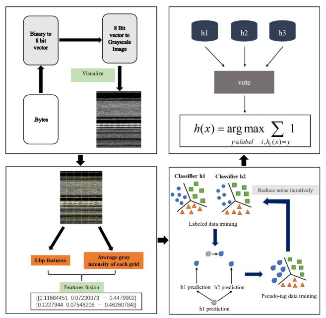
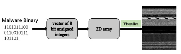
The traditional signature-based detection method requires detailed manual analysis to extract the signatures of malicious samples, and requires a large number of manual markers to maintain the signature library, which brings a great time and resource costs, and makes it difficult to adapt to the rapid generation and mutation of malware. Methods based on traditional machine learning often require a lot of time and resources in sample labeling, which results in a sufficient inventory of unlabeled samples but not directly usable. In view of these issues, this paper proposes an effective malware classification framework based on malware visualization and semi-supervised learning. This framework includes mainly three parts: malware visualization, feature extraction, and classification algorithm. Firstly, binary files are processed directly through visual methods, without assembly, decompression, and decryption; Then the global and local features of the gray image are extracted, and the visual image features extracted are fused on the whole by a special feature fusion method to eliminate the exclusion between different feature variables. Finally, an improved collaborative learning algorithm is proposed to continuously train and optimize the classifier by introducing features of inexpensive unlabeled samples. The proposed framework was evaluated over two extensively researched benchmark datasets, i.e., Malimg and Microsoft. The results show that compared with traditional machine learning algorithms, the improved collaborative learning algorithm can not only reduce the cost of sample labeling but also can continuously improve the model performance through the input of unlabeled samples, thereby achieving higher classification accuracy.

| [1] | A. P. Namanya, A. Cullen, I. U. Awan, J. P. Disso, The world of Malware: An overview, in 2018 IEEE 6th International Conference on Future Internet of Things and Cloud (FiCloud), 2018, pp. 420-427, doi: 10.1109/FiCloud.2018.00067. |
| [2] |
A. Martín, H. D. Menéndez, D. Camacho, MOCDroid: Multi-objective evolutionary classifier for Android malware detection, Soft. Comput., 21 (2017), 7405-7415. doi: 10.1007/s00500-016-2283-y

|
| [3] | P. Foran, Of digital reliance, risk and resilience, Progres. Railro., 62 (2019), 30-30, 32-33. |
| [4] |
K. Rieck, P. Trinius, C. Willems, T. Holz, Automatic analysis of malware behavior using machine learning, J. Comput. Secur., 19 (2011), 639-668. doi: 10.3233/JCS-2010-0410
|
| [5] | F. Touchette, The evolution of malware, Network Security, 1 (2016), 11-14. |
| [6] | D. Gavrilut, M. Cimpoesu, A. Dan, L. Ciortuz, Malware detection using machine learning, Int. Multiconfer. Comput. Sci. Inform. Tech., 2010. |
| [7] | L. Nataraj, S. Karthikeyan, G. Jacob, B. S. Manjunath, Malware images: Visualization and automatic classification, Proceedings of the 8th International Symposium on Visualization for Cyber Security (VizSec), 2011, Available from: https://doi.org/10.1145/2016904.2016908. |
| [8] | W. Huang, J. W. Stokes, MtNet: A multi-task neural network for dynamic Malware classification, International Conference on Detection of Intrusions and Malware, and Vulnerability Assessment, 2016. |
| [9] | J. Saxe, K. Berlin, Deep neural network based Malware detection using two dimensional binary program features, 2015 10th International Conference on Malicious and Unwanted Software (MALWARE), (2015), 11-20. |
| [10] | E. David, N. S. Netanyahu, DeepSign: Deep learning for automatic malware signature generation and classification, Internat. Joint Confer. Neural Networks, (2015), 1-8. |
| [11] | M. Ahmadi, D. Ulyanov, S. Semenov, M. Trofimov, G. Giacinto, Novel feature extraction, selection and fusion for effective Malware family classification, 6th ACM Conference on Data and Applications Security and Privacy (CODASPY), 2016. |
| [12] | Z. A. Genç, G. Lenzini, P. Y. A. Ryan, Next Generation Cryptographic Ransomware, (2018), 385-401. |
| [13] | J. Sahs, L. Khan, A machine learning approach to Android Malware detection, Intelligence and Security Informatics Conference (EISIC), (2012), 141-147. |
| [14] | X. G. Han, W. Qu, X. X. Yao, C. Y. Guo, F. Zhou, Research on malicious code variants detection based on texture fingerprint, J. Commun., 2014. |
| [15] |
K. S. Han, J. H. Lim, B. Kang, E. G. Im, Malware analysis using visualized images and entropy graphs, Int. J. Inf. Secur., 14 (2015), 1-14. doi: 10.1007/s10207-014-0242-0
|
| [16] | J. Y. Kim, S. J. Bu, S. B. Cho, Zero-day malware detection using transferred generative adversarial networks based on deep autoencoders, Inform. Ences, (2018), 83-102. |
| [17] | S. Shang, N. Zheng, X. Jian, M. Xu, H. P. Zhang, Detecting malware variants via function-call graph similarity, International Conference on Malicious & Unwanted Software, (2010), 113-120. |
| [18] | B. Anderson, C. Storlie, T. Lane, Improving malware classification: Bridging the static/dynamic gap, ACM Workshop on Security & Artificial Intelligence, 2012. |
| [19] | P. Zhang, B. Sun, R Ma, A Li, A novel visualization Malware detection method based on Spp-Net, 2019 IEEE 5th International Conference on Computer and Communications (ICCC), (2019), 510-514. |
| [20] |
G. Xiao, J. Li, Y. Chen, K. Li, MalFCS: An effective malware classification framework with automated feature extraction based on deep convolutional neural networks, J. Parall. Distribut. Comput., 141 (2020), 49-58. doi: 10.1016/j.jpdc.2020.03.012
|
| [21] |
J. E. Engelen, H. H. Hoos, A survey on semi-supervised learning, Mach. Learn., 109 (2020), 373-440. doi: 10.1007/s10994-019-05855-6
|
| [22] | K. Nigam, A. Mccallum, T. Mitchell, Semi-supervised text classification Using EM, MIT Press, (2006), 33-55. |
| [23] | F. D. Frumosu, M. Kulahci, Outliers detection using an iterative strategy for semi-supervised learning, Quality Reliab. Eng., 35 (2019). |
| [24] |
Z. H. Zhou, M. Li, Tri-training: Exploiting unlabeled data using three classifiers, IEEE Trans. Knowl. Data Eng., 17 (2005), 1529-1541. doi: 10.1109/TKDE.2005.186
|
| [25] | A. Blum, T. Mitchell, Combining labeled and unlabeled data with co-training, Proceed Conference Computer Learning, (1998), 92-100. |
| [26] | Y. Zhou, S. Goldman, Democratic co-learning, Proc. 16th IEEE Int. Conf. Tools Artif. Intell., (2004), 594-602. |
| [27] |
D. G. Kong, G. H. Yan, Discriminant malware distance learning on structural information for automated malware classification, Performance Evaluation Review, 41 (2013), 347-348. doi: 10.1145/2494232.2465531
|
| [28] | D. Angluin, P. Laird, Learning from noisy examples, Mach. Learn., 4 (1988), 343-370, Available from: https://doi.org/10.1007/BF00116829 |
| [29] | M. J. Sullivan, Distribution of edaphic diatoms in a mississippi salt marsh: A canonical correlation analysis, J. Phycol., (1982), 130-133. |
| [30] |
D. G. Lowe, Distinctive image features from scale-invariant keypoints, Int. J. Comput. Vision., 60 (2004), 91-110. doi: 10.1023/B:VISI.0000029664.99615.94
|
| [31] | N. Dalal, B. Triggs, Histograms of oriented gradients for human detection, IEEE Computer Society Conference on Computer Vision & Pattern Recognition (CVPR), 2005. |
| [32] | T. Ojala, M. Pietikäinen, T. Mäenpää, Gray scale and rotation invariant texture classification with local binary patterns, European Conference on Computer Vision (ECCV), (2000), 404-420. |
| [33] | J. Ma, X. Jiang, A. Fan, J. Jiang, J. Yan, Image matching from Handcrafted to deep features: A survey, Int. J. Comput. Vision, 1 (2020), 1-57. |
| [34] | T. Ahonen, J. Matas, H. Chu, M. Pietikäinen, Rotation invariant image description with local binary pattern histogram fourier features, Image Analys., (2009), 61-70. |
| [35] | H. Ran, W. Qi, Z. Guo, Feature reduction of multi-scale LBP for texture classification, 2015 International Conference on Intelligent Information Hiding and Multimedia Signal Processing (ⅡH-MSP), (2015), 397-400. |
| [36] | I. H. Witten, E. Frank, Data mining: Practical machine learning tools and techniques, Second Edition, ACM Sigmod. Record., 31 (2005), 76-77. |
| [37] |
M. Haghighat, M. Abdel-Mottaleb, W. Alhalabi, Fully automatic face normalization and single sample face recognition in unconstrained environments, Expert Syst Appl., 47(2016), 23-34. doi: 10.1016/j.eswa.2015.10.047
|
| [38] | R. Ronen, M. Radu, C. Feuerstein, E. Yom-Tov, M. Ahmadi, Microsoft Malware Classification Challenge, CORR, 2018. |


Figures(4) / Tables(8)

Tan Gao, Lan Zhao, Xudong Li, Wen Chen. Malware detection based on semi-supervised learning with malware visualization[J]. Mathematical Biosciences and Engineering, 2021, 18(5): 5995-6011. doi: 10.3934/mbe.2021300


 DownLoad: