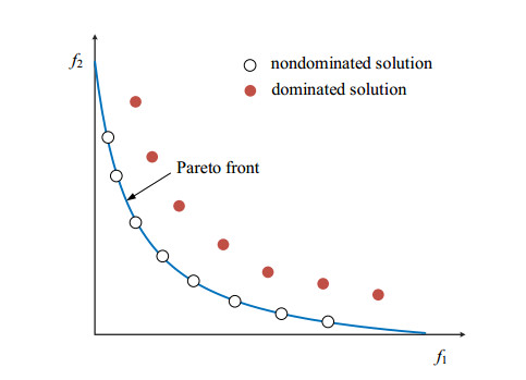
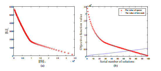
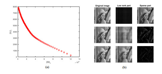
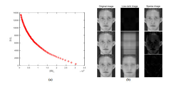
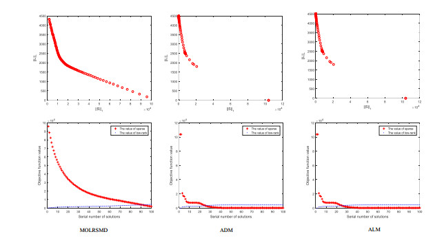
This paper addresses the problem of finding the low-rank and sparse components of a given matrix. The problem involves two conflicting objective functions, reducing the rank and sparsity of each part simultaneously. Previous methods combine two objectives into a single objective penalty function to solve with traditional numerical optimization approaches. The main contribution of this paper is to put forward a multiobjective method to decompose the given matrix into low-rank component and sparse part. We optimize two objective functions with an evolutionary multiobjective algorithm MOEA/D. Another contribution of this paper, a modified low-rank and sparse matrix model is proposed, which simplifying the variable of objective functions and improving the efficiency of multiobjective optimization. The proposed method obtains a set of solutions with different trade-off between low-rank and sparse objectives, and decision makers can choose one or more satisfied decomposed results according to different requirements directly. Experiments conducted on artificial datasets and nature images, show that the proposed method always obtains satisfied results, and the convergence, stability and robustness of the proposed method is acceptable.
Citation: Tao Wu, Yu Lei, Jiao Shi, Maoguo Gong. 2017: An evolutionary multiobjective method for low-rank and sparse matrix decomposition, Big Data and Information Analytics, 2(1): 23-37. doi: 10.3934/bdia.2017006
This paper addresses the problem of finding the low-rank and sparse components of a given matrix. The problem involves two conflicting objective functions, reducing the rank and sparsity of each part simultaneously. Previous methods combine two objectives into a single objective penalty function to solve with traditional numerical optimization approaches. The main contribution of this paper is to put forward a multiobjective method to decompose the given matrix into low-rank component and sparse part. We optimize two objective functions with an evolutionary multiobjective algorithm MOEA/D. Another contribution of this paper, a modified low-rank and sparse matrix model is proposed, which simplifying the variable of objective functions and improving the efficiency of multiobjective optimization. The proposed method obtains a set of solutions with different trade-off between low-rank and sparse objectives, and decision makers can choose one or more satisfied decomposed results according to different requirements directly. Experiments conducted on artificial datasets and nature images, show that the proposed method always obtains satisfied results, and the convergence, stability and robustness of the proposed method is acceptable.

| [1] |
Beck A., Teboulle M. (2009) A fast iterative shrinkage-thresholding algorithm for linear inverse problems. SIAM Journal on Imaging Sciences 2: 183-202. doi: 10.1137/080716542

|
| [2] |
Cai J.-F., Candès E. J., Shen Z. (2010) A singular value thresholding algorithm for matrix completion. SIAM Journal on Optimization 20: 1956-1982. doi: 10.1137/080738970
|
| [3] |
Cai Z., Wang Y. (2006) A multiobjective optimization-based evolutionary algorithm for constrained optimization. IEEE Transactions on Evolutionary Computation 10: 658-675. doi: 10.1109/TEVC.2006.872344
|
| [4] |
E. J. Candès, X. Li, Y. Ma and J. Wright, Robust principal component analysis?
Journal of the ACM (JACM), 58 (2011), Art. 11, 37 pp.
10.1145/1970392.1970395 MR2811000 |
| [5] |
Candès E. J., Recht B. (2009) Exact matrix completion via convex optimization. Foundations
of Computational Mathematics 9: 717-772. doi: 10.1007/s10208-009-9045-5
|
| [6] |
Chandrasekaran V., Sanghavi S., Parrilo P. A., Willsky A. S. (2011) Rank-sparsity incoherence for matrix decomposition. SIAM Journal on Optimization 21: 572-596. doi: 10.1137/090761793
|
| [7] |
C. A. C. Coello, D. A. Van~Veldhuizen and G. B. Lamont,
Evolutionary Algorithms for Solving Multi-Objective Problems, Genetic Algorithms and Evolutionary Computation, 5. Kluwer Academic/Plenum Publishers, New York, 2002.
10.1007/978-1-4757-5184-0 MR2011496 |
| [8] |
K. Deb,
Multi-objective Optimization Using Evolutionary Algorithms, John Wiley & Sons, Ltd. , Chichester, 2001.
MR1840619 |
| [9] |
Deb K., Pratap A., Agarwal S., Meyarivan T. (2002) A fast and elitist multiobjective genetic algorithm: NSGA-Ⅱ. IEEE Transactions on Evolutionary Computation 6: 182-197. doi: 10.1109/4235.996017
|
| [10] |
Fazel M., Hindi H., Boyd S. P. (2001) A rank minimization heuristic with application to minimum order system approximation. in Proceedings of the American Control Conference, IEEE 6: 4734-4739. doi: 10.1109/ACC.2001.945730
|
| [11] |
Gong M., Jiao L., Du H., Bo L. (2008) Multiobjective immune algorithm with nondominated neighbor-based selection. Evolutionary Computation 16: 225-255. doi: 10.1162/evco.2008.16.2.225
|
| [12] | Z. Lin, A. Ganesh, J. Wright, L. Wu, M. Chen and Y. Ma, Fast convex optimization algorithms for exact recovery of a corrupted low-rank matrix, Computational Advances in Multi-Sensor Adaptive Processing (CAMSAP), vol. 61,2009. |
| [13] | Z. Lin, M. Chen and Y. Ma, The augmented lagrange multiplier method for exact recovery of corrupted low-rank matrices, arXiv preprint, arXiv: 1009.5055, 2010. |
| [14] |
K. Miettinen,
Nonlinear Multiobjective Optimization, Kluwer Academic Publishers, Boston, MA, 1999.
MR1784937 |
| [15] | Qian C., Yu Y., Zhou Z.-H. (2015) Pareto ensemble pruning. in AAAI 2935-2941. |
| [16] | ————, Subset selection by pareto optimization, in Advances in Neural Information Processing Systems, (2015), 1774-1782. |
| [17] |
Recht B., Fazel M., Parrilo P. A. (2010) Guaranteed minimum-rank solutions of linear matrix equations via nuclear norm minimization. SIAM Review 52: 471-501. doi: 10.1137/070697835
|
| [18] | J. D. Schaffer, Multiple objective optimization with vector evaluated genetic algorithms, in Proceedings of the 1st international Conference on Genetic Algorithms. L. Erlbaum Associates Inc. , (1985), 93-100. |
| [19] |
Starck J. L., Elad M., Donoho D. L. (2005) Image decomposition via the combination of sparse representations and a variational approach. IEEE Transactions on Image Processing 14: 1570-1582. doi: 10.1109/TIP.2005.852206
|
| [20] |
Yan J., Liu J., Li Y., Niu Z., Liu Y. (2010) Visual saliency detection via rank-sparsity decomposition. in IEEE International Conference on Image Processing, IEEE 1089-1092. doi: 10.1109/ICIP.2010.5652280
|
| [21] | Yuan X., Yang J. (2013) Sparse and low-rank matrix decomposition via alternating direction methods. Pacific Journal of Optimization 9: 167-180. |
| [22] |
Zhang C., Liu J., Tian Q., Xu C., Lu H., Ma S. (2011) Image classification by non-negative
sparse coding, low-rank and sparse decomposition. IEEE Conference on Computer Vision and Pattern Recognition (CVPR) 1673-1680. doi: 10.1109/CVPR.2011.5995484
|
| [23] | Zhang Q., Li H. (2007) MOEA/D: A multiobjective evolutionary algorithm based on decomposition. IEEE Transactions on Evolutionary Computation 11: 712-731. |
| [24] | Zibulevsky M., Pearlmutter B. A. (2001) Blind source separation by sparse decomposition in a signal dictionary. Neural Computation 13: 863-882. |
| [25] | Zitzler E., Laumanns M., Thiele L., et al. (2001) SPEA2: Improving the strength pareto evolutionary algorithm. in Eurogen 3242: 95-100. |
Figures(8) / Tables(2)

Tao Wu, Yu Lei, Jiao Shi, Maoguo Gong. 2017: An evolutionary multiobjective method for low-rank and sparse matrix decomposition, Big Data and Information Analytics, 2(1): 23-37. doi: 10.3934/bdia.2017006


 DownLoad: