Stability and bifurcation analysis of a two-patch model with the Allee effect and dispersal

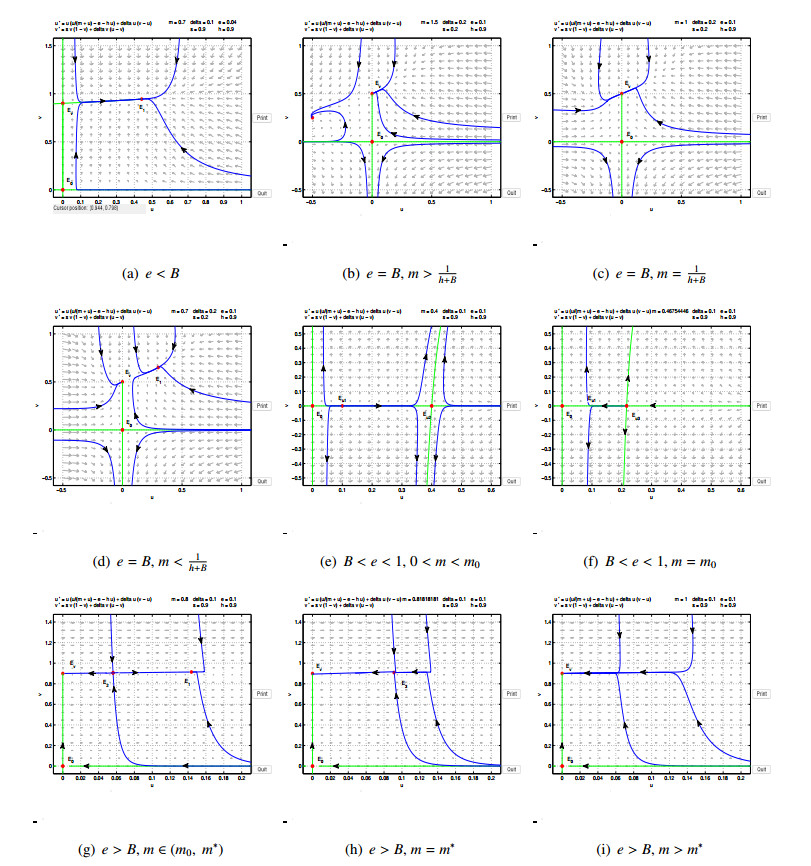
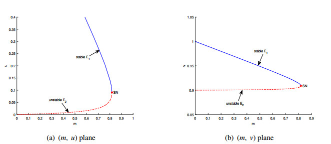
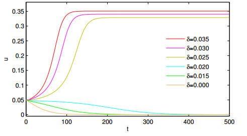
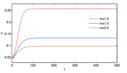
1.   Introduction

The conservation of biodiversity is a paramount issue of global scale ^[1]. One way to protect endangered species is to create nature reserves or "refuges" ^[2], where such species are safe and can breed healthy populations. Studies have shown that remote islands and mountainous regions often provide opportunities to protect endangered species ^[3]. However, the destruction of the natural habitat of many species due to human activities has resulted in fragmentation. Habitat fragmentation is defined as the breaking up of a large intact area of a single vegetation type into smaller intact units ^[4]. This leads to patch-level changes that can negatively impact species diversity ^[5,6,7,8]. Also note that dispersal strategies, which are necessary to estimate species success under fragmentation, are not well studied in the field ^[9]. For example, different dispersal speeds may change how easily a species can travel between patches or increase the likelihood of leaving resource-filled patches to avoid competition or predation ^[10]. Numerous studies have shown that building bridges between patches that allow groups to communicate with each other can help communities to endure ^[11,12]. Thus, studies of dispersal behavior, particularly between habitat patches are informative for the conservation of endangered species ^[13,14,15]. To this end, the linear diffusion model is well known. For example, in ^[16], the author proposed two models, i.e., with discrete patches,

and continuous patches,

where $D, \ a^j, \ b^j, \ a$ and $b$ are positive constants. In these models, linear diffusion means that the species can move randomly.

Notice that random movement is reasonable only in some cases (e.g., oceanic plankton ^[17]). Gurney and Nisbet ^[18] studied a biased random motion model as follows:

where $r$ is the intrinsic birth rate, $D_1$ is the random dispersal rate and $D_2$ is a positive constant depending upon the proportionality between the bias and density gradient. In this model, the authors suggest that the movement of individual populations is largely random, but is influenced to a small extent by the overall distribution of peers. The authors considered that members of a population walk pseudo-randomly in a rectangular network, and that the probability distribution of each step is slightly distorted by the local population density gradient; thus, the intensity of diffusion is $D_1\nabla ^2u+D_2\nabla \left(u\nabla u \right)$. Later, Allen ^[16] came up with a population modeled by pure biased diffusion, i.e., the discrete patches one

and continuous patches,

The biased diffusion model was formulated under the assumption that the population density affects the diffusion rate ^[19,20]. In other words, the diffusion rate is governed by the population density.

The Allee effect ^[21,22] plays an important role in population dynamics, and it can be divided into the strong Allee effect and weak Allee effect. And the strong Allee effect can lead to extinction. Liu et al. ^[23,24] studied the influence of strong and weak Allee effects on Leslie-Gower models. The additive Allee effect, i.e., an Allee effect involving both strong and weak Allee effect, can be written in the form

Lv et al. ^[25] studied the impact of the additive Allee effect on an SI epidemic model. In order to protect endangered species, it is particularly important to study the Allee effect in patch models. Chen et al. ^[26] studied the influence of the Allee effect of a two-patch model with linear dispersal:

where $a$ and $m$ are the Allee effect constants. $D_1$ and $D_2$ are dispersal rates of the two patches. Their study suggests that dispersal and the Allee effect may lead to the persistence or disappearance of the population in both patches. Wang ^[27] studied the global stability of the following two-patch models with the Allee effect:

Wang demonstrated that moderate dispersal to the better patch facilitates growth in total population density in the face of strong Allee effects. Many other scholars have studied the strong Allee effect and weak Allee effect ^{[28,29,30,31]}.

In ^[32], the authors proposed the following single-species model with the Allee effect:

where $r$ is the maximum birth rate, $A$ represents the strength of the Allee effect, $d$ is natural mortality and $b$ denotes the death rate due to intra-prey competition. It is well known that this type of Allee effect is the strong Allee effect, increasing the risk of extinction. It will be interesting to study the effects of diffusion on species via this Allee effect. As we know, there has been no study of the Allee effect in a two-patch model with nonlinear dispersal; thus for this motivation in this paper, we will study a two-patch model with the Allee effect and nonlinear dispersal as follows:

where $u$ and $v$ are the densities of the population in the first patch and the second patch, respectively. $A$ is the Allee effect constant. $r, d$ and $b$ are the birth rate, natural mortality and death rate due to intra-prey competition of the population in the first patch, respectively. $a$ and $c$ are the intrinsic growth rate and death rate due to intra-prey competition of the population in the second patch, respectively. $D$ is the dispersal coefficient.

It is worth mentioning that human intervention increased biodiversity in protected areas in spite of the Allee effect. Thus, in model (1.1), we assume that the population in first patch is affected by the Allee effect, while the population in the second patch is free of an Allee effect and is consistent with normal logistic growth. Moreover, it is well known that the natural habitats of many species are fragmented due to human intervention and exploitation. Thus, some patches are continuous while others are discrete; hence, it is important to consider both the ordinary differential equation (ODE) and partial differential equation (PDE) scenarios, while modeling such phenomenon.

As far as we are aware, this is the first time that both nonlinear dispersal and the Allee effect on the population dynamics of a species in a two-patch model have been considered. Although Wang has previously investigated the impace of the strong Allee effect in a patch model in ^[27], he did not consider the case in which diffusion between patches is nonlinear; thus, this article would be a good companion study to his research. By comparing the difference between nonlinear and linear dispersal, we conclude that nonlinear diffusion is more conducive to persistence in a fragmented environment.

The rest of this paper is organized as follows. In Section 2, the ODE case of model (2.1) is introduced. And in this section, the existence and stability of the equilibrium of model (2.1) are proved; the condition for saddle-node bifurcation to occur is proved and the impacts of the Allee effect and nonlinear dispersal are given. In Section 3, the PDE case of model (2.1) is introduced. And the impacts of Allee effect and nonlinear dispersal in PDE case are also given. We end this paper with a conclusion in Section 4.

2.   The ODE case

2.1.   Existence and stability of equilibrium

In order to simplify system (1.1), let

and

We still reserve $u$, $v$, $t$ to express $\bar{u}, \ \bar{v}, \ \tau$, respectively. Then, we get the following simplified system:

with the following initial conditions: $\ u\left(0 \right) \geq 0, \ v\left(0 \right) \geq 0.$ In the above equation, $0 < e < 1$ and $m$, $h$, $\delta$ and $s$ are all positive constants. The existence and stability of all nonnegative equilibria of model (2.1) are respectively proved as follows:

(ⅰ) The trivial equilibrium $E_0\left(0, \ 0 \right)$ and boundary equilibrium $E_v\left(0, \ \frac{s}{s+\delta} \right)$ always exist.

(ⅱ) The equilibrium $\bar E(\bar u, 0)$ exists on the $u$ coordinate axis where $\bar u$ satisfies the following equation:

If $m\ge \frac{1-e}{h+\delta}$, Eq (2.2) obviously has no positive root. In what follows, we investigate the case that $m < \frac{1-e}{h+\delta}$. Notice that the discriminant of Eq (2.2) is $\Delta_1(m) = (h+\delta)^2 m^2-2(1+e)(h+\delta)m+(1-e)^2$. The discriminant of $\Delta_1(m)$ is $\Delta_2 = 16e(h+\delta)^2 > 0$. Thus, $\Delta_1(m) = 0$ has two positive real roots:

From $0 < e < 1$, we can easily get that $m_0 < \frac{1-e}{h+\delta} < m_1$. Thus, if $m_0 < m < \frac{1-e}{h+\delta}$, it follows that $\Delta_1(m) < 0$; then, Eq (2.2) has no positive real root.

(ⅲ) Regarding the existence of the positive equilibrium point, from model (2.1) we know that the positive equilibrium $E\left(u, \ v \right)$ satisfies the following equation:

Denote $B = \frac{s\delta}{s+\delta}$. The above yields that

If $e = B$, Eq (2.3) becomes

Therefore, if $m\ge \frac{1}{h+B}$, there is no positive equilibrium; if $m < \frac{1}{h+B}$, Eq (2.4) has a unique positive real root. If $B < e < 1$, Eq (2.3) has a unique positive real root. In what follows, we investigate the case that $B < e < 1$. Notice that the discriminant of Eq (2.3) is $\varDelta _3\left(m \right) = \left(h+B \right) ^2m^2-2\left(e-B+1 \right) \left(h+B \right) m+\left(e-B-1 \right) ^2$. The discriminant of $\varDelta _3(m)$ is $\varDelta _4 = 16\left(e-B \right) \left(h+B \right) ^2 > 0$. Thus $\varDelta _3(m) = 0$ has two positive real roots:

From $B < e < 1$, we get that $m^* < \frac{1+B-e}{h+B} < m_{1}^{*}$. Therefore, if $m^* < m < \frac{1+B-e}{h+B}$, it follows that $\varDelta _3\left(m \right) < 0$; then, Eq (2.3) has no positive real root.

Theorem 2.1. 1) There are two equilibria on the positive coordinate axis of $u$: $E_{\bar{u}_1}\left(\bar{u}_1, \ 0 \right)$ and $E_{\bar{u}_2}\left(\bar{u}_2, \ 0 \right)$ when $0 < m < m_0$.

2) There is a unique equilibrium on the positive coordinate axis of $u$: $E_{\bar{u}_3}\left(\bar{u}, \ 0 \right)$ when $m = m_0$. And

Theorem 2.2. 1) If $e < B$, there is a unique positive equilibrium $E_1\left(u_1, \ v_1 \right)$.

2) If $e = B$, there is a unique positive equilibrium $E_1\left(u_1, \ v_1 \right)$ when $m < \frac{1}{h+B}$; there is no positive equilibrium when $m\ge \frac{1}{h+B}$.

3) If $B < e < 1$,

(i) there are two positive equilibria $E_1\left(u_1, \ v_1 \right)$ and $E_2\left(u_2, \ v_2 \right)$ when $m < m^*$;

(ii) there is a unique positive equilibrium $E_3\left(u_3, \ v_3 \right)$ when $m = m^*$;

(iii) there is no positive equilibrium when $m > m^*$. And

Next, we consider the local stability of the equilibrium point. The Jacobian matrix of system (2.1) at any point $E\left(u, \ v \right)$ is

where

Theorem 2.3. 1) $E_0\left(0, \ 0 \right)$ is always a saddle.

2) If $B < e < 1$, $E_v\left(0, \ \frac{s}{s+\delta} \right)$ is locally stable; if $e < B$, $E_v\left(0, \ \frac{s}{s+\delta} \right)$ is a saddle.

3) If $e = B$,

(i) $E_v\left(0, \ \frac{s}{s+\delta} \right)$ is an attracting saddle-node, and the parabolic sector is on the right half-plane when $m > \frac{1}{h+B}$;

(ii)$E_v\left(0, \ \frac{s}{s+\delta} \right)$ is an attracting saddle-node, and the hyperbolic sector is on the right half-plane when $m < \frac{1}{h+B}$;

(iii) $E_v$ is a stable node when $m = \frac{1}{h+B}$.

Proof. 1) From Eq (2.5), the Jacobian matrix at $E_0\left(0, \ 0 \right)$ is

it follows that $E_0\left(0, \ 0 \right)$ is a saddle.

2) The Jacobian matrix at $E_v\left(0, \ \frac{s}{s+\delta} \right)$ is

thus, $E_v\left(0, \ \frac{s}{s+\delta} \right)$ is a saddle when $e < B$, while $E_v\left(0, \ \frac{s}{s+\delta} \right)$ is locally stable when $e > B$.

3) If $e = B$, $J_{E_v\left(0, \ \frac{s}{s+\delta} \right)}$ has a unique zero eigenvalue. Let $U_1 = u$ and $\ V_1 = v-\frac{s}{s+\delta}$; model (2.1) can be transformed into the following system:

Applying the Taylor expansion of $\frac{1}{m+U_1}$ at the origin, it can be rewritten as

where $G\left(U_1 \right)$ denotes the power series with the term $U_{1}^{j}$ satisfying that $j > 3$. The Jacobian matrix of system (2.6) at the origin is

Then we make the following transformation:

model (2.6) becomes as follows:

where $G_1$ and $\ G_2$ denote the power series with term $x_{1}^{i}y_{1}^{j}$ satisfying that $i+j > 3$ and

If $m\left(h+B \right) > 1$ (or $m\left(h+B \right) < 1$), we can see that the coefficient of $x_{1}^{2}$ is greater than zero (or less than zero). Applying Theorem 7.1 in ^[33], we know that $E_v\left(0, \ \frac{s}{s+\delta} \right)$ is an attracting saddle-node, and the parabolic (hyperbolic) sector is on the right half-plane when $q_0 > 0$ $(q_0 < 0)$. If $q_0 = 0$, i.e., $m = \frac{1}{h+B}$, system (2.7) becomes as follows:

Then we can obtain the implicit function

where $G_3\left(x_1 \right)$ denotes the power series with the term $x_{1}^{i}$, $i > 3$. Then

where $G_4\left(x_1 \right)$ denotes the power series with the term $x_{1}^{i}$, $i > 3$ and $q_2\ne 0$. According to Theorem 7.1 in ^[33], and combining the previous time changes, it is clear that $E_v\left(0, \ \frac{s}{s+\delta} \right)$ is a stable node. □

Theorem 2.4. 1) Both $E_{\bar{u}_1}\left(\bar{u}_1, \ 0 \right)$ and $E_{\bar{u}_2}\left(\bar{u}_2, \ 0 \right)$ are unstable when $m < m_0$;

2) $E_{\bar{u}_3}\left(\bar{u}_3, \ 0 \right)$ is a repelling saddle-node.

Proof. From Eq (2.5), the Jacobian matrix at $E_{\bar{u}_i}$ is

1) $\theta _{1_i} = \bar{u}_i\left[\frac{m}{\left(m+\bar{u}_i \right) ^2}-\left(h+\delta \right) \right] \ne 0;\ \theta _{2_i} = s+\delta \bar{u}_i > 0$ are two eigenvalues of $J_{E_{\bar{u}_i}}, i = 1, 2.$ Therefore, both $E_{\bar{u}_1}$ and $E_{\bar{u}_2}$ are unstable.

2) If $m = m_0$, $J_{E_{\bar{u}_3}}$ has a unique zero eigenvalue. Let $U_2 = u-\bar{u}_3$ and $\ V_2 = v$; model (2.1) can be transformed into the following system:

Using the same method as in Theorem 2.3, system (2.8) can be transformed into a form similar to Eq (2.7). After a complicated calculation, we get that $q_0 = -\left(h+\delta \right) \frac{\sqrt{e}}{1-\sqrt{e}} < 0$. Applying Theorem 7.1 in ^[33], $E_{\bar{u}_3}\left(\bar{u}_3, \ 0 \right)$ is a repelling saddle node; Theorem 2.4 is proved. □

Theorem 2.5. 1) $E_1\left(u_1, \ v_1 \right)$ is stable.

2) $E_2\left(u_2, \ v_2 \right)$ is always a saddle.

3) $E_3\left(u_3, \ v_3 \right)$ is an attracting saddle-node.

Proof. 1) From Eq (2.5), the determinant and the trace of $J_{E_1}$ are, respectively,

After a simple calculation, we get that $Det\left(J_{E_1} \right) > 0$ and $\ Tr\left(J_{E_1} \right) < 0$; thus, $E_1$ is locally stable.

2) From Theorem 2.2, if $B < e < 1$ and $m < m^*$, then $E_2\left(u_2, \ v_2 \right)$ exists. The determinant of $J_{E_2}$ is

After a simple calculation, we get that $\left(m+u_2 \right) ^2-m\left(h+B \right) < 0$, which means that $Det\left(J_{E_2} \right) < 0$ and $E_2\left(u_2, \ v_2 \right)$ is a saddle.

3) When $B < e < 1$ and $m = m^*$, $E_3\left(u_3, \ v_3 \right)$ exists. Then $\gamma _1 = 0$ and $\gamma _2 = s+\delta u_3 > 0$ are two eigenvalues of $J_{E_3}$. Using the same method as in Theorem 2.3, we know that $E_3\left(u_3, \ v_3 \right)$ is an attracting saddle node; Theorem 2.5 is proved. □

The existence and stability conditions for all equilibria are given in Table 1.

Theorem 2.6. The boundary equilibrium $E_v\left(0, \ \frac{s}{s+\delta} \right)$ is globally asymptotically stable when $B < e < 1, \ m > m^*$.

Proof. For model (2.1), it is easy to know that $\left. \frac{\text{d}u}{\text{d}t} \right|_{u = 0} = 0, \ \left. \frac{\text{d}v}{\text{d}t} \right|_{v = 0} = 0,$ which means that $u = 0$ and $v = 0$ constitute the invariant set of model (2.1). Thus, all solutions of model (2.1) are nonnegative. Consider the following equations:

Applying the comparison theorem for differential equations, we establish the comparison equations:

From Theorem 3.2 in ^[13], there are positive constants $M_1$ and $T_1$ that yield that $N_i\left(t \right) \le M$ for $\forall t > T_1$, i = 1, 2. So all solutions of model (2.1) are uniformly bounded. From Theorems 2.3 and 2.4, $E_v$ is locally asymptotically stable and there is no positive equilibrium when $B < e < 1, \ m > m^*$. Therefore, there exist no limit cycle in the first quadrant. Thus $E_v\left(0, \frac{s}{s+\delta} \right)$ is globally asymptotically stable. The proof of Theorem 2.6 is finished. □

Theorem 2.7. The positive equilibrium $E_1\left(u_1, \ v_1 \right)$ is globally asymptotically stable when $e < B$ or $e = B$ and $m < \frac{1}{h+B}$.

Proof. From Theorems 2.3 and 2.5, the unique positive equilibrium $E_1\left(u_1, \ v_1 \right)$ is locally asymptotically stable and the boundary equilibrium $E_v\left(0, \ \frac{s}{s+\delta} \right)$ is unstable in the first quadrant when $e < B$ or $e = B$ and $m < \frac{1}{h+B}$. Consider the Dulac function $g\left(u, \ v \right) = \frac{1}{u^2v^2}$. Applying $e\le B < s$, we get

where $M = \frac{1}{\left(m+u \right) ^2v^2}+\delta \left(\frac{1}{u^2v}+\frac{1}{uv^2} \right) > 0$ and

Applying the Bendixson-Dulac discriminant, model (2.1) has no limit cycle in the first quadrant. Since the solution of system (2.1) is ultimately bounded, we have that $E_1\left(u_1, \ v_1 \right)$ is globally asymptotically stable; hence, the proof of Theorem 2.7 is finished. □

Remark 2.1. Theorem 2.6 shows that the level of the Allee constant $m$ has a large effect on the extinction of the population in the first patch when the intensity of dispersal is low. In detail, when $B < e$, i.e., $\delta < \frac{se}{s-e}(s > e),$ the species in the first patch will go extinct at any initial value when $m > m^*$. The ecological significance of this result is that when the intensity of dispersal is low, if the birth rate of the population in the first patch is affected by the strong Allee effect such that the population faces severe difficulties in finding mates, then it will not be able to avoid extinction. However, when the intensity of dispersal is large, i.e., $\delta > \frac{se}{s-e}(s > e)$ which implies that $B > e$, the species in both patches will be permanent even though the species in the first patch has a strong Allee effect. In other words, nonlinear dispersal can be beneficial to the survival of the species.

The phase diagram for model (2.1) is given in Figure 1 for the different parameter cases.

2.2.   Saddle-node bifurcation

From Theorem 2.2, model (2.1) has two positive equilibria $E_1\left(u_1, \ v_1 \right)$ and $E_2\left(u_2, \ v_2 \right)$ when $B < e < 1$ and $m < m^*$; However, if $m = m^*$, it has a unique positive equilibrium $E_3\left(u_3, \ v_3 \right)$. Saddle-node bifurcation may be induced at here.

Theorem 2.8. Saddle-node bifurcation arises at $E_3\left(u_3, \ v_3 \right)$ when $B < e < 1$ and $m = m^*$.

Proof. From Theorem 1.5, we get that $Det\left(J_{E_3} \right) = 0$ and $\ Tr\left(J_{E_3} \right) = -\left(B+\frac{2\delta ^2}{s+\delta} \right) u_3-s < 0$ when $B < e < 1$ and $m = m^*$. Then $J_{E_3}$ has the unique zero eigenvalue $\gamma _1$. Let

be the eigenvectors of $J_{E_3}$ and $J_{E_3}^{T}$ corresponding to a zero eigenvalue. Next, we have

where $F_1$ and $F_2$ are given in Eq (2.9). It is easy to get

Applying the Sotomayor theorem ^[34], system (2.1) will experience saddle-node bifurcation at $E_3\left(u_3, \ v_3 \right)$ when $B < e < 1$ and $m = m^*$; Theorem 2.8 is proved. □

Besides, saddle-node bifurcation also occurs at $E_{\bar{u}_3}\left(\bar{u}, \ 0 \right)$ when $m = m_0$, and its proof is analogous to Theorem 2.8; thus, we omit it here.

2.3.   Impacts of Allee effect and nonlinear dispersal

From Theorem 2.7, the positive equilibrium point $E_1\left(u_1, \ v_1 \right)$ is globally asymptotically stable when $e < B$ or $e = B$ and $m = \frac{1}{h+B}$. Then, the total population abundance is $T = u_1+v_1$, where $v_1 = \frac{s+\delta u_1}{s+\delta}$ and

After a simple derivative calculation, we get

where $C: = \left(h+B \right) -\frac{m}{\left(m+u_1 \right) ^2} > 0$. Thus we have that $\frac{\text{d}T}{\text{d}m} = \frac{\text{d}u_1}{\text{d}m}+\frac{\text{d}v_1}{\text{d}m} < 0$. The above yields that the stronger the Allee effect, the lower the total population density. Figure 2 is the bifurcation diagram for parameter $m$, which was obtained by using MatCont ^[35].

Consider the subsystem of model (2.1) without nonlinear dispersal:

For model (2.10), it is well known that when the Allee effect is strong, it can lead to population extinction under certain initial values. For example, in Figure 3, it can be seen that the population of patch 1 becomes extinct in the absence of dispersal. However, it becomes persistent with the increase of the dispersal coefficient $\delta$, which reflects the positive effect of dispersal here. In Figure 4, the Allee effect does not lead to extinction when the dispersal coefficient $\delta$ is large enough, which is completely different from the model in which the Allee effect may lead to extinction of the population. Therefore reasonable dispersal is necessary for the conservation of scarce animals.

In order to better understand the role of nonlinear dispersal, we will present some comparison between nonlinear dispersal and linear dispersal. We introduce the model with linear dispersal as follows.

For model (2.11), up to now, we cannot present the complete qualitative analysis such as the sufficient and necessary condition for the existence of a positive equilibrium. We will obtain two sufficient conditions which ensure that system (2.11) does not have a positive equilibrium and there is a unique positive equilibrium, respectively. And, the complete qualitative analysis will be our future work.

Theorem 2.9. For model (2.11), if $m\ge \frac{1}{h}, \ e > s$ and $\delta > \frac{es}{e-s}$, then there is no positive equilibrium and the trivial equilibrium $O\left(0, \ 0 \right)$ is globally asymptotically stable.

Proof. Let the right-hand sides of model (2.11) equal to zero to get

It is easy to obtain that $H_1\left(v \right)$ is strictly monotonically increasing and concave. And $H_1\left(0 \right) = 0, H_{1}^{'}\left(0 \right) = \frac{\delta -s}{\delta} > 0$ and $\ H_2\left(0 \right) = 0$. Besides, we can obtain

And if $h\geq\frac{1}{m}$, then

Thus $H_2\left(u \right)$ is also strictly monotonically increasing and concave. The above yields that if $H_{1}^{'}\left(0 \right) H_{2}^{'}\left(0 \right) > 1$, two curves $u = H_1(v)$ and $v = H_2(u)$ will not intersect each other in the first quadrant which implies that model (2.11) has no positive equilibrium. And the diagrams of curves $H_1\left(v \right)$ and $H_2\left(u \right)$ are shown in Figure 6. Notice that when $e > s$ and $\delta \ge \frac{es}{e-s}$, it follows that $H_{1}^{'}\left(0 \right) H_{2}^{'}\left(0 \right) > 1$.

Summarizing the above, we can conclude that $m\ge \frac{1}{h}$ and $\ e > s, \ \delta > \frac{es}{e-s}$, model (2.11) has no positive equilibrium, and it only has the trivial equilibrium $O\left(0, \ 0 \right)$.

Next, we will consider the local asymptotic stability of the trivial equilibrium $O\left(0, \ 0 \right)$ of model (2.11). The Jacobian matrix at $O\left(0, \ 0 \right)$ is

And

Therefore $O\left(0, \ 0 \right)$ is locally asymptotically stable. Also model (2.11) has no limit cycle since it has no positive equilibrium when $m\ge \frac{1}{h}, \ e > s$ and $\delta > \frac{es}{e-s}$. The above yields that $O\left(0, \ 0 \right)$ is globally asymptotically stable. Theorem 2.9 is proved. □

Theorem 2.9 shows that the impacts of nonlinear diffusion and linear diffusion are different. In detail, high nonlinear diffusion intensity can make the species in both patches coexist (see Figure 3), while high linear diffusion intensity causes the species in the first patch to become extinct (see Figure 5).

Theorem 2.10. For model (2.11), if $m\ge \frac{1}{h}$ and $0 < \delta \le s$, then a unique positive equilibrium $\hat{E}\left(\hat{u}, \ \hat{v} \right)$ exists, where $\hat{u}$ and $\hat{v}$ satisfy Eq (2.12). And $\hat{E}\left(\hat{u}, \ \hat{v} \right)$ is globally asymptotically stable when $0 < \delta < \frac{s-e}{2}$.

Proof. From the proof of Theorem 2.9, if $m\geq \frac{1}{h}$, we can obtain that both $H_1\left(v \right)$ and $H_2\left(u \right)$ are strictly monotonically increasing and concave for $u > 0$ and $v > 0$. From $H_1\left(\frac{s-\delta}{s} \right) = H_2\left(0 \right) = 0$ and $H_{1}^{'}\left(\frac{s-\delta}{s} \right) = \frac{s-\delta}{\delta}\ge 0, \ H_{2}^{'}\left(0 \right) > 0$, then two curves $u = H_1(v)$ and $v = H_2(u)$ will intersect each other once in the first quadrant which implies that model (2.1) has a unique positive equilibrium. This is shown in Figure 6 (b). And a simple calculation gives us $H_{1}^{'}\left(\hat{v} \right) H_{2}^{'}\left(\hat{u} \right) > 1$.

From Eq (2.13), we get $Det\left(J_O \right) = e\left(\delta -s \right) -\delta s < 0$. Thus $O\left(0, \ 0 \right)$ is a saddle. Next, we will consider the stability of the positive equilibrium $\hat{E}\left(\hat{u}, \ \hat{v} \right)$. From Eq (2.12), model (2.11) can rewritten as follows:

The Jacobian matrix at $\hat{E}\left(\hat{u}, \ \hat{v} \right)$ is

And

Therefore $\hat{E}\left(\hat{u}, \ \hat{v} \right)$ is locally asymptotically stable. Consider again the Dulac function $g\left(u, \ v \right) = \frac{1}{u^2v^2}$. Applying $\delta \le \frac{s-e}{2}$, we get

where $\bar{M} = \frac{1}{\left(m+u \right) ^2v^2}+\delta \left(\frac{1}{u^3v}+\frac{1}{uv^3} \right) > 0$. Using the Bendixson-Dulac discriminant in the same way in Theorem 2.7, we can see that $\hat{E}\left(\hat{u}, \ \hat{v} \right)$ is globally asymptotically stable. Theorem 2.10 is proved. □

Remark 2.2. In our manuscript, we focus on how dispersal can keep the species with an Allee effect from becoming extinct. In detail, From Theorem 2.7 and Remark 2.1, we conclude that for the model (1.2) with a nonlinear dispersal mechanism, a large amplitude of nonlinear dispersal can prevent the species with a strong Allee effect from going extinct. However, Theorem 2.9 states that if the diffusion between two patches is linear, the species in both patches may still go extinct when the Allee constant is large, even if the dispersal intensity is large. Theorem 2.10 states that if the diffusion between two patches is linear, the species in both patches can persist when the Allee constant is large and the dispersal intensity is less. Through a comparison of Theorem 2.7, Remark 2.1 and Theorems 2.9 and 2.10, it is not difficult to obtain that linear and nonlinear dispersal have different impaces on the species' permanence. In all, a large amplitude of nonlinear dispersal or less intensity of linear dispersal can keep the species with a strong Allee effect from becoming extinct. The above comparison of nonlinear diffusion with linear diffusion has theoretical and practical significance.

3.   The PDE case

In this section we will study the effect of dispersal rate $\delta$ for spatially explicit PDE versions of systems (2.1) and (2.11).

3.1.   Notations and preliminary observations

Lemma 3.1. Consider an $m\times m$ system of reaction-diffusion equations, where each equation is defined as follows: for all $i = 1, ..., m,$

where $d_i \in (0, +\infty)$, $f = (f_1, ..., f_m):\mathbb{R}^m \rightarrow \mathbb{R}^m$ is continuously differentiable on $\Omega$ and $u_{i0}\in L^{\infty}(\Omega)$. Then, there exists a time interval $T > 0$ within which a unique classical solution to Eq (3.1) exists, i.e., the solution is well-defined and smooth on $[0, T)$. Let $T^*$ be the maximum value for all such intervals $T$. It follows that

If the non-linearity $(f_i)_{1\leq i\leq m}$ is also quasi-positive, i.e., if

then

Lemma 3.2. Under the same notations and assumptions as in Lemma 3.1, let us consider an additional condition. Suppose that $f$ exhibits at most polynomial growth and there exist ${\bf b}\in \mathbb{R}^m$ and a lower triangular invertible matrix $P$ with nonnegative entries such that for any $r \in [0, +\infty)^m,$ we have

Then, for any initial value $u_0 \in L^{\infty}(\Omega, \mathbb{R}_+^m),$ the system (3.1) admits a strong global solution.

Based on the given assumptions, it is widely recognized that the following local existence result, originally presented by D. Henry in ^[36], holds true:

Theorem 3.1. The system (3.1) possesses a unique and classical solution $(u, v)$ defined over the interval $[0, T_{\max}]\times \Omega$. If $T_{\max} < \infty$, then

where $T_{\max }$ denotes the eventual blow-up time in $\mathbb{L}^{\infty }(\Omega).$

3.2.   A case of linear dispersal

Consider the following spatially explicit PDE version of the linear dispersal system motivated by ODE system $(2.11)$, resulting in the following reaction diffusion system, defined on $\Omega = [0, L]$:

Here

In this framework the patch structure is in a simple one dimensional domain $[0, L]$, where the region from $[0, L_{1}]$ is where the population is subject to an Allee effect, and the region from $[L_{1}, L]$ is where the population is not subject to an Allee effect. Here linear dispersal is assumed for the populations modeled by the standard Laplacian operator.

One can typically think of the species $u$ as the population starting in the $[0, L_{1}]$ patch, where it is subject to an Allee effect and will move via linear dispersal into the $[L_{1}, L]$ patch. Once it enters this patch, it is no longer subject to an Allee effect. Similarly we can think of the species $v$ as the population starting in the $[L_{1}, L]$ patch, where there is no Allee effect in place. However it moves into the $[0, L_{1}]$ patch via linear dispersal and upon entering this patch, it is immediately subject to an Allee effect. We consider the problem in the spatial dimension $n = 1$. Also the above mentioned functions $m(x), m_{1}(x), h(x), h_{1}(x), s(x), s_{1}(x), e(x)$ and $e_{1}(x)$ are all assumed to be in $L^{\infty}[0, L]$. We can state the following result.

Lemma 3.3. Consider the reaction diffusion system (3.3); then, there exist global in time non-negative classical solutions to this system, for certain positive bounded initial data.

Proof. The non-negativity of solutions follows via the quasi-positivity of the right-hand-side of Eq (3.3). Next, via a simple comparison for the $u$ equation we have,

This follows by using the positivity of the parameter $m$. Comparison with the logistic equation, via the use of Lemma 3.2 yields the result. The analysis for the $v$ equation follows similarly. □

3.3.   A case of non-linear dispersal

Consider the following spatially explicit version of nonlinear dispersal system $(2.1)$, resulting in the following reaction diffusion system, defined on $\Omega = [0, L]$:

In this framework the patch structure is in a simple one dimensional domain $[0, L]$, where the region from $[0, L_{1}]$ is where the population is subject to an Allee effect, and the region from $[L_{1}, L]$ is where the population is not subject to an Allee effect. Here nonlinear dispersal is assumed for the populations modeled by a non-standard Laplacian operator. We consider the problem in the spatial dimension $n = 1$. Again the functions $m(x), m_{1}(x), h(x), h_{1}(x), s(x), s_{1}(x), e(x)$ and $e_{1}(x)$ are all assumed to be nonnegative functions in $L^{\infty}[0, L]$. Furthermore, since the $s(x), h(x)$ functions have to mimic the $h, s$ parameters from the ODE systems considered earlier, we assume that there exists a positive constant $C_{1}$ such that $0 < C_{1} < \min(h(x), h_{1}(x), s(x), s_{1}(x))$.

We state the following result.

Theorem 3.2. Consider the reaction diffusion system (3.5); then, there exist global in time nonnegative classical solutions to this system for certain positive bounded initial data.

Proof. Consider the $u$ equation for the reaction diffusion system (3.5). Dividing through by $u$ we obtain, the following equivalent equation:

This follows by formally dividing through by $u$ and $v$ assuming positivity. Integrating the above equation over $\Omega$ yields,

From this, it follows that

It follows, by using the earlier estimate on the right-hand-side of the $u$ equation in Lemma 3.3, that $0 < C_{1} < \min(h(x), h_{1}(x), s(x), s_{1}(x))$. Now, by using the inequality $\log(x) < x, x > 0$, we obtain

An application of the Gronwall inequality yields

Similar analysis follows for the $v$ equation. Thus the $L^{1}(\Omega)$ norms of the $\log(u)$ cannot blow-up at any finite time $T^{*} < \infty$ for suitable initial data $u_{0}(x)$ such that the $\log(u_{0}(x))$ is well defined. This in turn yields control of the $L^{1}(\Omega)$ norms of the solution. Here $C_{2}$ is a pure constants that could absorb the other parameters in the problem. This, in conjunction with classical theory ^[36], where essentially one needs to control the right-hand-side of Eq (3.5) in $L^{p}$ for $p > \frac{n}{2}$, yields the result. □

3.4.   Numerical simulations

The numerical simulations for both the linear Eq (3.3) and nonlinear Eq (3.5) in the context of dispersal PDEs were executed by using MATLAB R2021b. The simulations employed the built-in function $\verb|pdepe|$, specifically designed to solve one-dimensional parabolic and elliptic PDEs. The spatial domain was set as the unit-sized interval $[0, 1]$, which was discretized into $100$ sub-intervals. It has been numerically validated under some parametric restrictions, and for some given data, a large magnitude of nonlinear dispersal or less intensity of linear dispersal may prevent species impacted by the Allee effect from becoming extinct (See Figures 5–13).

4.   Conclusions

In this paper, the interplay of the Allee effect and nonlinear dispersal in a two-patch model have been studied. Our goal was to determine whether nonlinear diffusion between the two patches contributes to overcoming the Allee effect.

When the dispersal intensity is low, we have concluded that a population $u$ will go extinct when $B < e < 1$ and $m > m^*$. Besides, we also proved that the two positive equilibrium points $E_1\left(u_1, \ v_1 \right)$ and $E_2\left(u_2, \ v_2 \right)$ of model (2.1) will undergo saddle-node bifurcation when $m = m^*$. These findings suggest that the Allee effect has a major impact on the extinction of the population in patch 1 when the dispersal intensity is very weak. However, the positive equilibrium $E_1\left(u_1, \ v_1 \right)$ is always globally asymptotically stable when $e < B$, i.e., $\delta > \frac{se}{s-e}$. The above result shows that both species will persist when the nonlinear dispersal intensity is high. In other words, under large nonlinear dispersal, the persistence of both species seems independent of the Allee effect.

Besides, for the corresponding model with linear dispersal, we have obtained two interesting results corresponding to when the Allee effect is strong. The results show that when the linear dispersal is high, both species will go extinct. However, the species with low linear dispersal will persist. We declare that a large magnitude of nonlinear dispersal or a lower intensity of linear dispersal may prevent species with a strong Allee effect from becoming extinct.

The above are results derived in the ODE case. We have derived analogous results in the PDE case as well. Herein, we set up a one dimensional domain to have two explicit patches, i.e., one patch in which the populations are subject to an Allee effect and the other patch in which they are not. The species move in and out of these patches via linear diffusion, as well as nonlinear diffusion. What we observe in the PDE case is that high nonlinear diffusion can eliminate the impact of the strong Allee effect so that populations do not become extinct; see Figures 11–13. This complements the ODE model's findings for continuous patch models. We also observe that, in the case of linear diffusion, a low intensity of diffusion can also lead to coexistence. This again is in accordance with our ODE findings. This is also true, even if we take an initial condition in the patch that is subject to an Allee effect, such that the $||u_{0}||_{\infty} < M$, that is the peak of the initial data is below the Allee threshold. Thus the small linear diffusion allows the species to disperse into the second patch, and escape the Allee effect before it can cause local extinction; see Figure 10.

Another important use of the PDE model is its applications to habitat fragmentation due to human intervention and exploitation. Some fragmented patches are large while others are small in area. Although ODE models with a patch structure are powerful, all in all they are not spatially explicit and thus cannot capture this effect of patches of different sizes. They cannot explicitly model the case of a patch, which is actually say 10, 20 or 30 percent of the entire domain. However, in the PDE case with a patch structure we can model this situation. We included this in our simulations in the PDE case. You will see that we attempted patches which are both one-third the size of the entire domain and 1/2 the size of the domain. We note that in both cases we can obtain coexistence. Thus patch size does not seem to play a part in achieving the coexistence dynamics; one can see this by comparing Figures 11–13 or Figures 7 and 8. Proving this rigorously will make for very interesting future work.

Recent studies by Srivastava et al. ^[37] and Chen et al. ^[38] have inspired further exploration. These studies investigate the impact of fear in a purely competitive two-species model, where one species instills fear in the other. To advance our understanding, it would be valuable to enhance future research by extending the incorporation of the fear effect into both linear and nonlinear dispersal systems, considering both ODE and PDE formulations. In summary, future investigations that modify the ODE and PDE versions of linear and nonlinear dispersal systems to incorporate the fear effect build upon recent work and have the potential to deepen our understanding of ecological dynamics. By exploring the role of fear in species interactions, we can uncover new dimensions and pave the way for more accurate modeling and conservation approaches. Other future directions in the PDE cases will include investigating edge effects with a patch structure ^[39] and investigating blow-up prevention with patches ^[40,41].

As is known, the traditional growth rate of species is logistic and an Allee effect in place may cause a species to become extinct. To this end it is interesting to propose a model with two patches, i.e., one where there is logistic growth and the other where there is an Allee effect. Thus, in this manuscript, we have explored a suitable dispersal strategy which can benefit species in both patches. In other words, we discuss the rolet of dispersal in keeping the species subject to an Allee effect from extinction. Our results show that a large magnitude of nonlinear dispersal or a lower intensity of linear dispersal may prevent species that are subject to a strong Allee effect from becoming extinct. We point out that it is also meaningful to investigate a two patch model, where the form of the Allee effect in the various patches could change, such as a strong effect in one patch versus a weak effect in the other patch. We leave such an investigation for future work.

Use of AI tools declaration

The authors declare that they have not used artificial intelligence tools in the creation of this article.

Acknowledgment

This work was supported by the National Natural Science Foundation of China (11601085) and the Natural Science Foundation of Fujian Province (2021J01614, 2021J01613).

Conflict of interest

The authors declare that there is no conflict of interest.