Allee effect-driven complexity in a spatiotemporal predator-prey system with fear factor

Yuhong Huo; Gourav Mandal; Lakshmi Narayan Guin; Santabrata Chakravarty; Renji Han; Yuhong Huo; Gourav Mandal; Lakshmi Narayan Guin; Santabrata Chakravarty; Renji Han

doi:10.3934/mbe.2023834

Mathematical Biosciences and Engineering

2023, Volume 20, Issue 10: 18820-18860. doi: 10.3934/mbe.2023834

Previous Article Next Article

Research article

Allee effect-driven complexity in a spatiotemporal predator-prey system with fear factor

1.
School of Finance and Mathematics, Huainan Normal University, Dongshanxi Street, Huainan, 232038, China
2.
Department of Mathematics, Visva-Bharati, Santiniketan 731235, India
3.
Former Professor, Department of Mathematics, Visva-Bharati, Santiniketan 731235, India
4.
School of Science, Zhejiang University of Science and Technology, Hangzhou 310023, China

Academic Editor: Peter Kim

Received: 25 July 2023 Revised: 19 September 2023 Accepted: 20 September 2023 Published: 09 October 2023

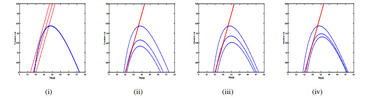
In this paper, we propose a spatiotemporal prey-predator model with fear and Allee effects. We first establish the global existence of solution in time and provide some sufficient conditions for the existence of non-negative spatially homogeneous equilibria. Then, we study the stability and bifurcation for the non-negative equilibria and explore the bifurcation diagram, which revealed that the Allee effect and fear factor can induce complex bifurcation scenario. We discuss that large Allee effect-driven Turing instability and pattern transition for the considered system with the Holling-Ⅰ type functional response, and how small Allee effect stabilizes the system in nature. Finally, numerical simulations illustrate the effectiveness of theoretical results. The main contribution of this work is to discover that the Allee effect can induce both codimension-one bifurcations (transcritical, saddle-node, Hopf, Turing) and codimension-two bifurcations (cusp, Bogdanov-Takens and Turing-Hopf) in a spatiotemporal predator-prey model with a fear factor. In addition, we observe that the circular rings pattern loses its stability, and transitions to the coldspot and stripe pattern in Hopf region or the Turing-Hopf region for a special choice of initial condition.
- reaction-diffusion system,
- fear and Allee effect,
- normal form,
- center manifold theory,
- bifurcation theory,
- spatiotemporal pattern transition
Citation: Yuhong Huo, Gourav Mandal, Lakshmi Narayan Guin, Santabrata Chakravarty, Renji Han. Allee effect-driven complexity in a spatiotemporal predator-prey system with fear factor[J]. Mathematical Biosciences and Engineering, 2023, 20(10): 18820-18860. doi: 10.3934/mbe.2023834

Related Papers:

Abstract

In this paper, we propose a spatiotemporal prey-predator model with fear and Allee effects. We first establish the global existence of solution in time and provide some sufficient conditions for the existence of non-negative spatially homogeneous equilibria. Then, we study the stability and bifurcation for the non-negative equilibria and explore the bifurcation diagram, which revealed that the Allee effect and fear factor can induce complex bifurcation scenario. We discuss that large Allee effect-driven Turing instability and pattern transition for the considered system with the Holling-Ⅰ type functional response, and how small Allee effect stabilizes the system in nature. Finally, numerical simulations illustrate the effectiveness of theoretical results. The main contribution of this work is to discover that the Allee effect can induce both codimension-one bifurcations (transcritical, saddle-node, Hopf, Turing) and codimension-two bifurcations (cusp, Bogdanov-Takens and Turing-Hopf) in a spatiotemporal predator-prey model with a fear factor. In addition, we observe that the circular rings pattern loses its stability, and transitions to the coldspot and stripe pattern in Hopf region or the Turing-Hopf region for a special choice of initial condition.

References

[1]	F. Courchamp, T. Clutton-Brock, B. Grenfell, Inverse density dependence and the Allee effect, Trend. Ecol. Evol., 14 (1999), 405–410. https://doi.org/10.1016/S0169-5347(99)01683-3 doi: 10.1016/S0169-5347(99)01683-3
[2]	P. A. Stephens, W. J. Sutherland, R. P. Freckleton, What is the Allee effect, Oikos, 87 (1999), 185–190. https://doi.org/10.2307/3547011 doi: 10.2307/3547011
[3]	P. A. Stephens, W. J. Sutherland, Consequences of the Allee effect for behaviour, ecology and conservation, Trends Ecol. Evol., 14 (1999), 401–405. https://doi.org/10.1016/s0169-5347(99)01684-5 doi: 10.1016/s0169-5347(99)01684-5
[4]	F. Courchamp, L. Berec, J. Gascoigne, Allee Effects in Ecology and Conservation, Oxford University Press, Oxford, 2008. https://doi.org/10.1093/acprof:oso/9780198570301.001.0001
[5]	D. Scheel, C. Packer, Group hunting behavior of lions: a search for cooperation, Anim. Behav., 41 (1991), 697–709. https://doi.org/10.1016/S0003-3472(05)80907-8 doi: 10.1016/S0003-3472(05)80907-8
[6]	M. T. Alves, F. M. Hilker, Hunting cooperation and Allee effects in predators, J. Theor. Biol., 419 (2017), 13–22. https://doi.org/10.1016/j.jtbi.2017.02.002 doi: 10.1016/j.jtbi.2017.02.002
[7]	R. Han, G. Mandal, L. N. Guin, S. Chakravarty, Dynamical response of a reaction-diffusion predator-prey system with cooperative hunting and prey refuge, J. Stat. Mech., 2022 (2022), 103502. https://doi.org/10.1088/1742-5468/ac946d doi: 10.1088/1742-5468/ac946d
[8]	L. Y. Zanette, A. F. White, M. C. Allen, M. Clinchy, Perceived predation risk reduces the number of offspring songbirds produce per year, Science, 334 (2011), 1398–1401. https://doi.org/10.1126/science.1210908 doi: 10.1126/science.1210908
[9]	X. Y. Wang, L. Y. Zanette, X. F. Zou, Modelling the fear effect in predator-prey interaction, J. Math. Biol., 73 (2016), 1179–1204. https://doi.org/10.1007/s00285-016-0989-1 doi: 10.1007/s00285-016-0989-1
[10]	P. A. Schmidt, L. D. Mech, Wolf pack size and food acquisition, Am. Nat., 150 (1997), 513–517. https://doi.org/10.1086/286079 doi: 10.1086/286079
[11]	F. Courchamp, D. W. Macdonald, Crucial importance of pack size in the African wild dog Lycaon pictus, Anim. Conserv., 4 (2001), 169–174. https://doi.org/10.1017/S1367943001001196 doi: 10.1017/S1367943001001196
[12]	S. Vinoth, R. Sivasamy, K. Sathiyanathan, B. Unyong, G. Rajchakit, R. Vadivel, et al., The dynamics of a Leslie type predator-prey model with fear and Allee effect, Adv. Differ. Equ., 2021 (2021), 1–22. https://doi.org/10.1186/s13662-021-03490-x doi: 10.1186/s13662-021-03490-x
[13]	B. Dennis, Allee effects: population growth, critical density, and the chance of extinction, Nat. Resour. Model., 3 (1989), 481–538. https://doi.org/10.1111/j.1939-7445.1989.tb00119.x doi: 10.1111/j.1939-7445.1989.tb00119.x
[14]	A. D. Bazykin, Nonlinear Dynamics of Interacting Populations, World Scientific Publishing Company Incorporated, Singapore, 1998.
[15]	F. Courchamp, B. T. Grenfell, T. H. Clutton-Brock, Impact of natural enemies on obligately cooperative breeders, Oikos, 91 (2000), 311–322. https://doi.org/10.1034/j.1600-0706.2000.910212.x doi: 10.1034/j.1600-0706.2000.910212.x
[16]	A. Kent, C. P. Doncaster, T. Sluckin, Consequences for predators of rescue and Allee effects on prey, Ecol. Modell., 162 (2003), 233–245. https://doi.org/10.1016/S0304-3800(02)00343-5 doi: 10.1016/S0304-3800(02)00343-5
[17]	S. Zhou, Y. Zhou, G. Wang, The stability of predator-prey systems subject to the Allee effects, Theor. Popul. Biol., 67 (2005), 23–31. https://doi.org/10.1016/j.tpb.2004.06.007 doi: 10.1016/j.tpb.2004.06.007
[18]	K. H. Elliott, G. S. Betini, D. R. Norris, Fear creates an Allee effect: experimental evidence from seasonal populations, Proc. R. Soc. B Biol. Sci., 284 (2017), 20170878. https://doi.org/10.1098/rspb.2017.0878 doi: 10.1098/rspb.2017.0878
[19]	S. K. Sasmal, Population dynamics with multiple Allee effects induced by fear factors-A mathematical on prey-predator interactions, Appl. Math. Modell., 64 (2018), 1–14. https://doi.org/10.1016/j.apm.2018.07.021 doi: 10.1016/j.apm.2018.07.021
[20]	Y. Li, M. He, Z. Li, Dynamics of a ratio-dependent Leslie-Gower predator-prey model with Allee effect and fear effect, Math. Comput. Simul., 201 (2022), 417–439. https://doi.org/10.1016/j.matcom.2022.05.017 doi: 10.1016/j.matcom.2022.05.017
[21]	Y. Shi, J. H. Wu, Q. Cao, Analysis on a diffusive multiple Allee effects predator-prey model induced by fear factors, Nonlinear Anal. Real World Appl., 59 (2021), 103249. https://doi.org/10.1016/j.nonrwa.2020.103249 doi: 10.1016/j.nonrwa.2020.103249
[22]	L. Y. Lai, Z. L. Zhu, F. D. Chen, Stability and bifurcation analysis in a predator-prey model with the additive Allee effect and the fear effect, Mathematics, 8 (2020), 1280. https://doi.org/10.3390/math8081280 doi: 10.3390/math8081280
[23]	J. P. Suraci, M. Clinchy, L. M. Dill, D. Roberts, L. Y. Zanette, Fear of large carnivores causes a trophic cascade, Nat. Commun., 7 (2016), 10698. https://doi.org/10.1038/ncomms10698 doi: 10.1038/ncomms10698
[24]	X. Wang, X. Zou, Modeling the fear effect in predator-prey interactions with adaptive avoidance of predators, Bull. Math. Biol., 79 (2017), 1325–1359. https://doi.org/10.1007/s00285-016-0989-1 doi: 10.1007/s00285-016-0989-1
[25]	A. J. Wirsing, W. J. Ripple, A comparison of shark and wolf research reveals similar behavioral responses by prey, Front. Ecol. Environ., 9 (2011), 335–341. https://doi.org/10.1890/090226 doi: 10.1890/090226
[26]	M. J. Sheriff, C. J. Krebs, R. Boonstra, The sensitive hare: sublethal effects of predator stress on reproduction in snowshoe hares, J. Anim. Ecol., 78 (2009), 1249–1258. https://doi.org/10.1111/j.1365-2656.2009.01552. doi: 10.1111/j.1365-2656.2009.01552
[27]	J. Wang, Y. Cai, S. Fu, W. Wang, The effect of the fear factor on the dynamics of a predator-prey model incorporating the prey refuge, Chaos: Interdiscip. J. Nonlinear Sci., 29 (2019), 083109. https://doi.org/10.1063/1.5111121 doi: 10.1063/1.5111121
[28]	S. Samaddar, M. Dhar, P. Bhattacharya, Effect of fear on prey-predator dynamics: Exploring the role of prey refuge and additional food, Chaos: Interdiscip. J. Nonlinear Sci., 30 (2020), 063129. https://doi.org/10.1063/5.0006968 doi: 10.1063/5.0006968
[29]	B. F. Xie, Z. C. Zhang, Impact of Allee and fear effects in a fractional order prey-predator system incorporating prey refuge, Chaos: Interdiscip. J. Nonlinear Sci., 33 (2023), 013131. https://doi.org/10.1063/5.0130809 doi: 10.1063/5.0130809
[30]	J. Liu, Qualitative analysis of a diffusive predator-prey model with Allee and fear effects, Int. J. Biomath., 14 (2021), 2150037. https://doi.org/10.1142/S1793524521500376 doi: 10.1142/S1793524521500376
[31]	D. Pal, D. Kesh, D. Mukherjee, Qualitative study of cross-diffusion and pattern formation in Leslie-Gower predator-prey model with fear and Allee effects, Chaos, Solitons Fractals, 167 (2023), 113033. https://doi.org/10.1016/j.chaos.2022.113033 doi: 10.1016/j.chaos.2022.113033
[32]	H. Amann, Dynamic theory of quasilinear parabolic equations Ⅱ. reaction-diffusion systems, Differ. Integr. Equations, 3 (1990), 13–75. https://doi.org/10.57262/die/1371586185 doi: 10.57262/die/1371586185
[33]	H. Amann, Dynamics theory of quasilinear parabolic systems Ⅲ. Global existence, Math. Z., 202 (1989), 219–250. https://doi.org/10.1007/BF01215256 doi: 10.1007/BF01215256
[34]	H. Amann, Nonhomogeneous linear and quasiliear elliptic and parabolic boundary value problems, in Function Spaces, Differential Operators and Nonlinear Analysis (eds. H.J. Schmeisser and H. Triebel), Teubner-Texte zur Mathematik, 133 (1993), 9–126. https://doi.org/10.1007/978-3-663-11336-2_1
[35]	S. L. Hollis, R. H. Martin, M. Pierre, Global existence and boundedness in reaction-diffusion systems, SIAM J. Math. Anal., 18 (1987), 744–761. https://doi.org/10.1137/0518057 doi: 10.1137/0518057
[36]	S. Wiggins, Introduction to Applied Nonlinear Dynamical Systems and Chaos, Springer, New York, 2003.
[37]	L. Perko, Differential Equations and Dynamical Systems, Springer-Verlag, New York, 2001.
[38]	Y. A. Kuznetsov, Elements of Applied Bifurcation Theory, Springer-Verlag, New York, 1998.
[39]	W. Govaerts, Y. A. Kuznetsov, H. G. E. Meijer, B. Al-Hdaibat, V. De Witte, A. Dhooge, et al., MATCONT: Continuation toolbox for ODEs in Matlab, Universiteit Gent, Belgium, 2019.
[40]	M. G. Crandall, P. H. Rabinowitz, Bifurcation from simple eigenvalues, J. Funct. Anal., 8 (1971), 321–340. https://doi.org/10.1016/0022-1236(71)90015-2 doi: 10.1016/0022-1236(71)90015-2
[41]	F. Q. Yi, J. J. Wei, J. P. Shi, Bifurcation and spatiotemporal patters in a homogeneous diffusive predator-prey system, J. Differ. Equations, 246 (2009), 1944–1977. https://doi.org/10.1016/j.jde.2008.10.024 doi: 10.1016/j.jde.2008.10.024
[42]	R. Han, S. Dey, M. Banerjee, Spatio-temporal pattern selection in a prey-predator model with hunting cooperation and Allee effect in prey, Chaos, Solitons Fractals, 171 (2023), 113441. https://doi.org/10.1016/j.chaos.2023.113441 doi: 10.1016/j.chaos.2023.113441
[43]	A. Morozov, S. Petrovskii, B. L. Li, Spatiotemporal complexity of patchy invasion in a predator-prey system with the Allee effect, J. Theor. Biol., 238 (2006), 18–35. https://doi.org/10.1016/j.jtbi.2005.05.021 doi: 10.1016/j.jtbi.2005.05.021
[44]	P. R. Chowdhury, S. Petrovskii, M. Banerjee, Oscillation and pattern formation in a slow-fast prey-predator system, Bull. Math. Biol., 83 (2021), 1–41. https://doi.org/10.1007/s11538-021-00941-0 doi: 10.1007/s11538-021-00941-0
[45]	S. Chow, C. Li, D. Wang, Normal Forms and Bifurcation of Plannar Vector Fields, Cambridge University Press, 1994. https://doi.org/10.1017/CBO9780511665639

Reader Comments

Your name:*

Email:*
© 2023 the Author(s), licensee AIMS Press. This is an open access article distributed under the terms of the Creative Commons Attribution License (http://creativecommons.org/licenses/by/4.0)