A negative correlation ensemble transfer learning method for fault diagnosis based on convolutional neural network

Long Wen; Liang Gao; Yan Dong; Zheng Zhu; Long Wen; Liang Gao; Yan Dong; Zheng Zhu

doi:10.3934/mbe.2019165

Mathematical Biosciences and Engineering

2019, Volume 16, Issue 5: 3311-3330. doi: 10.3934/mbe.2019165

Previous Article Next Article

Research article Special Issues

A negative correlation ensemble transfer learning method for fault diagnosis based on convolutional neural network

1.
The State Key Laboratory of Digital Manufacturing Equipment & Technology, School of Mechanical Science & Engineering, Huazhong University of Science & Technology, Wuhan, 430074, China
2.
School of Electronic Information & Communications, Huazhong University of Science & Technology, Wuhan, 430074, China
3.
Department of Pathology, Longgang Central Hospital of Shenzhen City, Guangdong, 518116, China

Received: 23 January 2019 Accepted: 10 April 2019 Published: 17 April 2019

With the development of the smart manufacturing, data-driven fault diagnosis has receiving more and more attentions from both academic and engineering fields. As one of the most important data-driven fault diagnosis method, deep learning (DL) has achieved remarkable applications. However, the DL based fault diagnosis methods still have the following two drawbacks: 1) One of the most major branch of deep learning is to construct the deeper structures, however the deep learning models in fault diagnosis is very shadow. 2) As stated by the no-free-lunch theorem, no single model can perform best on every dataset, and the individual deep learning model still suffers from the generalization ability. In this research, a new negative correlation ensemble transfer learning method (NCTE) is proposed. Firstly, the transfer learning based ResNet-50 is proposed to construct a deep learning structure that has 50 layers. Secondly, several fully-connected layers and softmax classifiers are trained cooperatively using negative correlation learning (NCL). Thirdly, the hyper-parameters of the proposed NCTE are determined by cross validation. The proposed NCTE is conducted on the KAT Bearing Dataset, and the prediction accuracy of NCTE is as high as 98.73%. This results show that NCTE has achieved a good results compared with other machine learning and deep learning method.
- negative correlation learning,
- transfer learning,
- ensemble learning,
- convolutional neural network,
- fault diagnosis
Citation: Long Wen, Liang Gao, Yan Dong, Zheng Zhu. A negative correlation ensemble transfer learning method for fault diagnosis based on convolutional neural network[J]. Mathematical Biosciences and Engineering, 2019, 16(5): 3311-3330. doi: 10.3934/mbe.2019165

Related Papers:

Abstract

With the development of the smart manufacturing, data-driven fault diagnosis has receiving more and more attentions from both academic and engineering fields. As one of the most important data-driven fault diagnosis method, deep learning (DL) has achieved remarkable applications. However, the DL based fault diagnosis methods still have the following two drawbacks: 1) One of the most major branch of deep learning is to construct the deeper structures, however the deep learning models in fault diagnosis is very shadow. 2) As stated by the no-free-lunch theorem, no single model can perform best on every dataset, and the individual deep learning model still suffers from the generalization ability. In this research, a new negative correlation ensemble transfer learning method (NCTE) is proposed. Firstly, the transfer learning based ResNet-50 is proposed to construct a deep learning structure that has 50 layers. Secondly, several fully-connected layers and softmax classifiers are trained cooperatively using negative correlation learning (NCL). Thirdly, the hyper-parameters of the proposed NCTE are determined by cross validation. The proposed NCTE is conducted on the KAT Bearing Dataset, and the prediction accuracy of NCTE is as high as 98.73%. This results show that NCTE has achieved a good results compared with other machine learning and deep learning method.

References

[1]	L. Wen, Y. Dong and L. Gao, A new ensemble residual convolutionalneural network for remaining useful life estimation, Math. Biosci. Eng., 16 (2019), 862–880.
[2]	H. D. Shao, H. K. Jiang, X. Zhang, et al., Rolling bearing fault diagnosis using an optimization deepbelief network, Meas. Sci. Tech., 26 (2015), 115002.
[3]	R. Zhao, R. Yan, Z. Chen, et al., Deep learning and itsapplications to machine health monitoring: A survey. arXiv preprint arXiv:1612.07640, 2016.
[4]	M. Cerrada, R. V. Sánchez, C. Li, et al., A review on data-driven fault severityassessment in rolling bearings, Mech. Syst. Signal Proc., 99 (2018), 169–196.
[5]	Y. Bengio, A. Courville and P. Vincent, Representation learning: a review and new perspectives, IEEE T. Pattern Anal. Mach. Intell., 35 (2013), 1798–1828.
[6]	L. Wen, L. Gao and X. Y. Li, A new deep transfer learning based on sparseauto-encoder for fault diagnosis, IEEE T.Syst. Man Cybern. Syst., 49 (2019), 136–144.
[7]	J. L. Wang, J. Zhang and X. X. Wang, A data driven cycle time prediction with featureselection in a semiconductor wafer fabrication system, IEEE T. Semicond. Manuf., 31 (2018), 173–182.
[8]	S. Shao, S. McAleer, R. Yan, et al., Highly-accuratemachine fault diagnosis using deep transfer learning, IEEE T. Ind. Inform., 15 (2019), 2446–2455.
[9]	Z. Y. Wang, C. Lu and B. Zhou, Fault diagnosis for rotary machinery with selectiveensemble neural networks, Mech. Syst.Signal Proc., 113 (2018), 112–130.
[10]	D. H. Wolpert and W. G.Macready, No free lunch theorems for optimization, IEEE T. Evol. Comput., 1 (1997), 67–82.
[11]	H. Y. Sang, Q. K. Pan, J. Q. Li, et al., Effectiveinvasive weed optimization algorithms for distributed assembly permutationflowshop problem with total flowtime criterion, Swarm Evol. Comput., 44 (2019), 64–73.
[12]	X. Y. Li, C. Lu, L. Gao, et al., An Effective Multi-Objective Algorithm forEnergy Efficient Scheduling in a Real-Life Welding Shop, IEEE T. Ind. Inform., 14 (2018), 5400–5409.
[13]	J. Yosinski, J. Clune, Y. Bengio, et al., How transferable arefeatures in deep neural networks? In Advances in neural information processingsystems, (2014), 3320–3328.
[14]	L. Wen, X. Y. Li and L. Gao, A New Two-level Hierarchical Diagnosis Network based onConvolutional Neural Network, IEEE T.Instrum. Meas., (2019).
[15]	H. Y. Sang, Q. K. Pan, P. Y. Duan, et al., Aneffective discrete invasive weed optimization algorithm for lot-streamingflowshop scheduling problems. J. Intell.Manuf., 29 (2018), 1337–1349.
[16]	X.Y. Li, L. Gao, Q. Pan, et al., An effectivehybrid genetic algorithm and variable neighborhood search for integratedprocess planning and scheduling in a packaging machine workshop. IEEE Trans. Syst. Man Cybern. Syst., (2018).
[17]	K. Tidriri, N. Chatti, S. Verron, et al., Bridging data-driven andmodel-based approaches for process fault diagnosis and health monitoring: Areview of researches and future challenges, Annu.Rev. Control, 42 (2016), 63–81.
[18]	Z. Y. Yin and J. Hou, Recent advances on SVMbased fault diagnosis and process monitoring in complicated industrialprocesses, Neurocomputing, 174 (2016), 643–650.
[19]	J. Zheng, L. Gao, H. B. Qiu, et al., Difference mapping methodusing least square support vector regression for variable-fidelityapproximation modelling, Eng. Optimiz., 47 (2015), 719–736.
[20]	T. Han, D. Jiang, Q. Zhao, et al., Comparison of random forest,artificial neural networks and support vector machine for intelligent diagnosisof rotating machinery, Trans. Inst. Meas.Control, (2017), 1–13.
[21]	B. Cai, L. Huang and M. Xie, Bayesian networks in fault diagnosis, IEEE T. Ind. Inform., 13 (2017), 2227–2240.
[22]	L. Wen, L. Gao and X. Y. Li, A new snapshot ensemble convolutional neuralnetwork for fault diagnosis, IEEE Access, 7 (2019), 32037–32047.
[23]	F. Wang, H. K. Jiang, H. D. Shao, et al., An adaptive deepconvolutional neural network for rolling bearing fault diagnosis, Meas. Sci. Technol., 28 (2017), 9.
[24]	J. L. Wang, J. Zhang and X. X. Wang, Bilateral LSTM: Atwo-dimensional long short-term memory model with multiply memory units forshort-term cycle time forecasting in re-entrant manufacturing systems. IEEE T. Ind. Inform., 14 (2018), 748–758.
[25]	J. Pan, Y. Zi, J. Chen, et al., LiftingNet: A novel deep learningnetwork with layerwise feature learning from noisy mechanical data for faultclassification, IEEE T. Ind. Inform., 65 (2018), 4973–4982.
[26]	S. B. Li, G. K. Liu, X. H. Tang, et al., An ensemble deepconvolutional neural network model with improved ds evidence fusion for bearingfault diagnosis, Sensors, 17 (2017), 1729.
[27]	C. Lu, Z. Y. Wang and B. Zhou, Intelligent fault diagnosis of rolling bearing using hierarchicalconvolutional network based health state classification, Adv. Eng. Inform., 32 (2017), 139–151.
[28]	B. Zhang, W. Li, X. Li, et al., Intelligent fault diagnosis undervarying working conditions based on domain adaptive convolutional neural networks, IEEE Access, 6 (2018), 66367–66384.
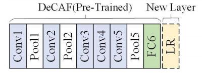
[29]	J. Donahue, Y. Q. Jia, O, Vinyals, et al., Decaf: A deepconvolutional activation feature for generic visual recognition, Internationalconference on machine learning, (2014),647–655.
[30]	R. Ren, T. Hung and K. C. Tan, A generic deep-learning-based approach for automatedsurface inspection, IEEE T. Cybern., 48 (2018), 929–940.
[31]	J. Wehrmann, G. S. Simoes and R. C. Barros, et al., Adultcontent detection in videos with convolutional and recurrent neural networks, Neurocomputing, 272 (2017), 432–438.
[32]	H. C. Shin, H. R. Roth, M. C. Gao, et al., Deep convolutionalneural networks for computer-aided detection: CNN architectures, datasetcharacteristics and transfer learning, IEEET. Med. Imaging, 35 (2016), 1285–1298.
[33]	E. Rezende, G. Ruppert, T. Carvalho, et al., Malicious softwareclassification using transfer learning of ResNet-50 deep neural network, 201716th IEEE International Conference on Machine Learning and Applications (ICMLA), (2017), 1011–1014.
[34]	O. Janssens, R. Walle, M. Loccufier, et al., Deep learning forinfrared thermal image based machine health monitoring. IEEE-ASME Trans. Mechatron., 23 (2018), 151–159.
[35]	Y. Zhou, W. C. Yi, L. Gao, et al., Adaptive differential evolution with sortingcrossover rate for continuous optimization problems. IEEE T. Cybern., 47 (2017), 2742–2753.
[36]	H. Y. Sang, P. Y. Duan and J. Q. Li, An effective invasive weed optimization algorithm forscheduling semiconductor final testing problem. Swarm Evol. Comput., 38 (2018), 42–53.
[37]	L. K. Hansen and P. Salamon, Neural network ensembles, IEEE T. Pattern Anal. Mach. Intell., 12 (1999), 993–1001.
[38]	H. H. Chen and X. Yao, Regularized negative correlation learning for neuralnetwork ensembles, IEEE T. Neural Netw., 20 (2009), 1962–1979.
[39]	J. C. Fernández, M. Cruz-Ramírez and C. Hervás-Martínez, Sensitivityversus accuracy in ensemble models of artificial neural networks frommulti-objective evolutionary algorithms. NeuralComput. Appl., 30 (2018), 289–305.
[40]	C. Hu, B. D. Youn, P. Wang, et al., Ensemble of data-drivenprognostic algorithms for robust prediction of remaining useful life, Reliab. Eng. Syst. Saf., 1 (2012), 120–35.
[41]	Z. Wu, W. Lin and Y. Ji, An integrated ensemble learning model for imbalanced faultdiagnostics and prognostics. IEEE Access, 6 (2018), 8394–8402.
[42]	U. P. Chong, Signal model-based fault detection and diagnosis forinduction motors using features of vibration signal in two-dimension domain. Strojniski Vestn. J. Mech. Eng., 57 (2011), 655–666.
[43]	L. Wen, X. Y. Li, L. Gao, et al., A new convolutional neuralnetwork based data-driven fault diagnosis method, IEEE Trans. Ind. Electron., 65 (2018), 5990–5998.
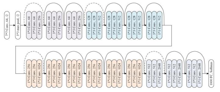
[44]	K. M. He, X.Y. Zhang, S. Q. Ren, et al., Deep residuallearning for image recognition, IEEE Conference on Computer Vision and PatternRecognition, (2016),770–778.
[45]	K. M. He, X. Y. Zhang, S. Q. Ren, et al., Delving deep into rectifiers: Surpassing human-level performanceon ImageNet classification. IEEEInternational Conference on Computer Vision, (2015),1026–1034.
[46]	M. Xiao, L. Wen, X. Li, et al., Modelingof the feed-motor transient current in end milling by using varying-coefficientmodel. Math. Probl. Eng., (2015).
[47]	S. Arlot and A. Celisse, A survey ofcross-validation procedures for model selection, Statistics surveys, 4 (2010), 40–79.
[48]	I. H. Witten, E. Frank, M. A. Hall, et al., Data Mining: Practical machinelearning tools and techniques. Morgan Kaufmann, (2016).
[49]	C. Lessmeier, J. K. Kimotho, D. Zimmer, et al., Conditionmonitoring of bearing damage in electromechanical drive systems by using motorcurrent signals of electric motors: A benchmark data set for data-drivenclassification. European Conference of the Prognostics and Health ManagementSociety, 05-08, (2016).
[50]	T. Han, D. Jiang, Q. Zhao, et al., Comparison of random forest, artificial neural networks andsupport vector machine for intelligent diagnosis of rotating machinery. Trans. Inst. Meas. Control, (2017), 1–13.
[51]	Y. H. Chen, G. L. Peng, C. H. Xie, et al., ACDIN: Bridging the gapbetween artificial and real bearing damages for bearing fault diagnosis, Neurocomputing, 294 (2018), 61–71.
[52]	Z. Y. Zhu, G. L. Peng, Y. H. Chen, et al., A convolutional neuralnetwork based on a capsule network with strong generalization for bearing faultdiagnosis, Neurocomputing, 323 (2019), 62–75.

Reader Comments

Your name:*

Email:*
© 2019 the Author(s), licensee AIMS Press. This is an open access article distributed under the terms of the Creative Commons Attribution License (http://creativecommons.org/licenses/by/4.0)