MAET-SAM: Magneto-Acousto-Electrical Tomography segmentation network based on the segment anything model

Shuaiyu Bu; Yuanyuan Li; Guoqiang Liu; Yifan Li; Shuaiyu Bu; Yuanyuan Li; Guoqiang Liu; Yifan Li

doi:10.3934/mbe.2025022

Mathematical Biosciences and Engineering

2025, Volume 22, Issue 3: 585-603. doi: 10.3934/mbe.2025022

Previous Article Next Article

Research article

MAET-SAM: Magneto-Acousto-Electrical Tomography segmentation network based on the segment anything model

1.
State Grid Beijing Electric Power Company, Beijing 100031, China
2.
Institute of Electrical Engineering, Chinese Academy of Sciences, Beijing 100190, China
3.
School of Electronic Electrical and Communication Engineering, University of Chinese Academy of Sciences, Beijing 100049, China
4.
China Railway Communication and Signal Survey & Design Co., Beijing 100036, China

Academic Editor: Yang Kuang

Received: 03 December 2023 Revised: 07 February 2024 Accepted: 01 March 2024 Published: 25 February 2025

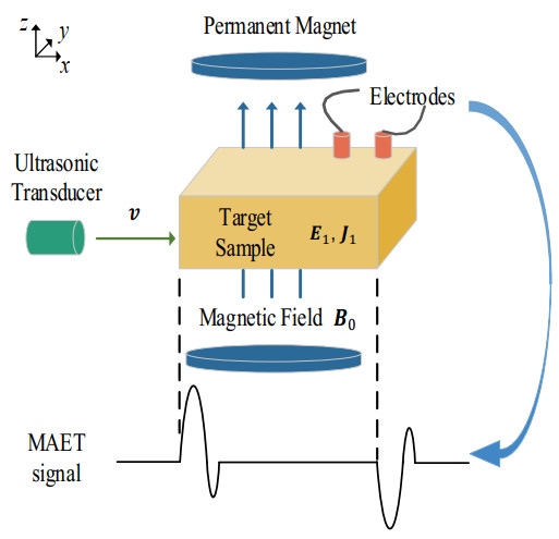
Magneto-Acousto-Electrical Tomography (MAET) is a hybrid imaging method that combines advantages of ultrasound imaging and electrical impedance tomography to image the electrical conductivity of biological tissues. In practical applications, different tissue or disease organization display various conductivity traits. However, the conductivity map consists of overlapping signals measured at multiple locations, the reconstruction results are affected by noise, which results in blurred reconstruction boundaries, low contrast, and irregular artifact distributions. To improve the image resolution and reduce noise of MAET, a dataset of conductivity maps reconstructed from MAET was established, dubbed MAET-IMAGE. Based on this dataset, we proposed a MAET tomography segmentation network based on the Segment Anything Model (SAM), termed as MAET-SAM. Specifically, we froze the encoder weights of SAM to extract rich feature information of image and design, an adaptive decoder with no prompts. In the end, an end-to-end segmentation model for specific MAET images with MAET-IMAGE was proposed. Qualitative and quantitative experiments demonstrated that MAET-SAM outperformed traditional segmentation methods and segmentation models with initial weights in terms of MAET image segmentation performance, bringing new breakthroughs and advancements to the field of medical imaging analysis and clinical diagnosis.
- MAET,
- image segmentation,
- segment anything model (SAM)
Citation: Shuaiyu Bu, Yuanyuan Li, Guoqiang Liu, Yifan Li. MAET-SAM: Magneto-Acousto-Electrical Tomography segmentation network based on the segment anything model[J]. Mathematical Biosciences and Engineering, 2025, 22(3): 585-603. doi: 10.3934/mbe.2025022

Related Papers:

Abstract

Magneto-Acousto-Electrical Tomography (MAET) is a hybrid imaging method that combines advantages of ultrasound imaging and electrical impedance tomography to image the electrical conductivity of biological tissues. In practical applications, different tissue or disease organization display various conductivity traits. However, the conductivity map consists of overlapping signals measured at multiple locations, the reconstruction results are affected by noise, which results in blurred reconstruction boundaries, low contrast, and irregular artifact distributions. To improve the image resolution and reduce noise of MAET, a dataset of conductivity maps reconstructed from MAET was established, dubbed MAET-IMAGE. Based on this dataset, we proposed a MAET tomography segmentation network based on the Segment Anything Model (SAM), termed as MAET-SAM. Specifically, we froze the encoder weights of SAM to extract rich feature information of image and design, an adaptive decoder with no prompts. In the end, an end-to-end segmentation model for specific MAET images with MAET-IMAGE was proposed. Qualitative and quantitative experiments demonstrated that MAET-SAM outperformed traditional segmentation methods and segmentation models with initial weights in terms of MAET image segmentation performance, bringing new breakthroughs and advancements to the field of medical imaging analysis and clinical diagnosis.

References

[1]	X. Song, Y. Xu, F. Dong, R. S. White, An instrumental electrode configuration for 3-D ultrasound modulated electrical impedance tomography, IEEE Sens. J. , 17 (2017), 8206–8214. https://doi.org/10.1109/JSEN.2017.2706758 doi: 10.1109/JSEN.2017.2706758
[2]	P. Grasland-Mongrain, C. Lafon, Review on biomedical techniques for imaging electrical impedance, IRBM, 39 (2018), 243–250. https://doi.org/10.1016/j.irbm.2018.06.001 doi: 10.1016/j.irbm.2018.06.001
[3]	H. Wen, J. Shah, R. S. Balaban, Hall effect imaging, IEEE Trans. Biomed. Eng. , 45 (1998), 119–124. https://doi.org/10.1109/10.650364 doi: 10.1109/10.650364
[4]	H. Wen, R. S. Balaban, The potential for hall effect breast imaging, Breast Dis. , 10 (1998), 191–195. https://doi.org/10.3233/BD-1998-103-418 doi: 10.3233/BD-1998-103-418
[5]	T. M. Deserno, H. Handels, K. H. Maier-Hein, S. Mersmann, C. Palm, T. Tolxdorff, Viewpoints on medical image processing: from science to application, Curr. Med. Imaging, 9 (2013), 79–88. https://doi.org/10.2174/1573405611309020002 doi: 10.2174/1573405611309020002
[6]	D. L. Pham, C. Xu, J. L. Prince, Current methods in medical image segmentation, Ann. Rev. Biomed. Eng. , 2 (2000), 315–337. https://doi.org/10.1146/annurev.bioeng.2.1.315 doi: 10.1146/annurev.bioeng.2.1.315
[7]	R. Wang, T. Lei, R. Cui, B. Zhang, H. Meng, A. K. Nandi, Medical image segmentation using deep learning: A survey. IET Image Process. , 16 (2022), 1243–1267. https://doi.org/10.1049/ipr2.12419 doi: 10.1049/ipr2.12419
[8]	A. Kirillov, E. Mintun, N. Ravi, H. Mao, C. Rolland, L. Gustafson, et al., Segment anything, in Proceedings of the IEEE/CVF International Conference on Computer Vision (ICCV), (2023), 4015–4026. https://doi.org/10.1109/ICCV51070.2023.00371
[9]	A. Montalibet, J. Jossinet, A. Matias, Scanning electric conductivity gradients with ultrasonically-induced Lorentz force, Ultrason. Imaging, 23 (2001), 117–132. https://doi.org/10.1177/016173460102300204 doi: 10.1177/016173460102300204
[10]	S. Haider, A. Hrbek, Y. Xu, Magneto-acousto-electrical tomography: A potential method for imaging current density and electrical impedance, Phys. Meas. , 29 (2008), S41. https://doi.rog/10.1088/0967-3334/29/6/S04 doi: 10.1088/0967-3334/29/6/S04
[11]	P. Grasland-Mongrain, J. M. Mari, J. Y. Chapelon, C. Lafon, Lorentz force electrical impedance tomography, IRBM, 34 (2013), 357–360. https://doi.org/10.1016/j.irbm.2013.08.002 doi: 10.1016/j.irbm.2013.08.002
[12]	L. Guo, G. Liu, H. Xia, Magneto-acousto-electrical tomography with magnetic induction for conductivity reconstruction, IEEE Trans. Biomed. Eng. , 62 (2015), 2114–2124. https://doi.org/10.1109/TBME.2014.2382562 doi: 10.1109/TBME.2014.2382562
[13]	L. Guo, G. F. Liu, Y. J. Yang, G. Q. Liu, Vector based reconstruction method in Magneto-Acousto-Electrical Tomography with magnetic induction, Chin. Phys. Lett. , 32 (2015), 094301. https://doi.org/10.1088/0256-307X/32/9/094301 doi: 10.1088/0256-307X/32/9/094301
[14]	L. Kunyansky, C. P. Ingram, R. S. Witte, Rotational magneto-acousto-electric tomography (MAET): theory and experimental validation, Phys. Med. Biol. , 62 (2017), 3025. https://doi.org/10.1088/1361-6560/aa6222 doi: 10.1088/1361-6560/aa6222
[15]	M. Dai, X. Chen, M. Chen, H. Lin, F. Li, S. Chen, A novel method to detect interface of conductivity changes in Magneto-Acousto-Electrical tomography using chirp signal excitation method, IEEE Access, 6 (2018), 33503–33512. https://doi.org/10.1109/ACCESS.2018.2841991 doi: 10.1109/ACCESS.2018.2841991
[16]	M. Dai, X. Chen, M. Chen, H. Lin, F. Li, S. Chen, A 2D magneto-acousto-electrical tomography method to detect conductivity variation using multifocus image method, Sensors, 18 (2018), 2373. https://doi.org/10.3390/s18072373 doi: 10.3390/s18072373
[17]	Z. F. Yu, Y. Zhou, Y. Z. Li, Q. Y. Ma, G. P. Guo, J. Tu, Performance improvement of magneto-acousto-electrical tomography for biological tissues with sinusoid-Barker coded excitation, Chin. Phys. B, 27 (2018), 094302. https://doi.org/10.1088/1674-1056/27/9/094302 doi: 10.1088/1674-1056/27/9/094302
[18]	T. Sun, X. Zeng, P. Hao, C. T. Chin, M. Chen, J. Yan, et al., Optimization of multi-angle magneto-acousto-electrical tomography (MAET) based on a numerical method, Math. Biosci. Eng. , 17 (2020), 2864–2880. https://doi.org/10.3934/mbe.2020161 doi: 10.3934/mbe.2020161
[19]	D. Deng, T. Sun, L. Yu, Y. Chen, X. Chen, M. Chen, et al., Image quality improvement of magneto-acousto-electrical tomography with Barker coded excitation, Biomed. Signal Process. Control, 77 (2022), 103823. https://doi.org/10.1016/j.bspc.2022.103823 doi: 10.1016/j.bspc.2022.103823
[20]	P. Li, W. Chen, G. Guo, J. Tu, D. Zhang, Q. Ma, General principle and optimization of magneto-acousto-electrical tomography based on image distortion evaluation, Med. Phys. , 50 (2023), 3076–3091. https://doi.org/10.1002/mp.16317 doi: 10.1002/mp.16317
[21]	Y. Li, S. Bu, X. Han, H. Xia, W. Ren, G. Liu, Magneto-acousto-electrical tomography with nonuniform static magnetic field, IEEE Trans. Instrum. Meas. , 72 (2023), 1–12. https://doi.org/10.1109/TIM.2023.3244814 doi: 10.1109/TIM.2023.3244814
[22]	P. K. Sahoo, S. Soltani, A. K. C. Wong, A survey of thresholding techniques, Comput. Vis. Graph Image Process. , 41 (1998), 233–260. https://doi.org/10.1016/0734-189X(88)90022-9 doi: 10.1016/0734-189X(88)90022-9
[23]	J. K. Udupa, S. Samarasekera, Fuzzy connectedness and object definition: Theory, algorithms, and applications in image segmentation, Graph Models Image Process. , 58 (1996), 246–261. https://doi.org/10.1006/gmip.1996.0021 doi: 10.1006/gmip.1996.0021
[24]	P. Arbelaez, M. Maire, C. Fowlkes, J. Malik, Contour detection and hierarchical image segmentation, IEEE Trans. Pattern Anal. Mach. Intell. , 33 (2010), 898–916. https://doi.org/10.1109/TPAMI.2010.161 doi: 10.1109/TPAMI.2010.161
[25]	D. Shen, G. Wu, H. I. Suk, Deep learning in medical image analysis, Ann. Rev. Biomed. Eng. , 19 (2017), 221–248. https://doi.org/10.1146/annurev-bioeng-071516-044442 doi: 10.1146/annurev-bioeng-071516-044442
[26]	Q. Huang, H. Tian, L. Jia, Z. Li, Z. Zhou, A review of deep learning segmentation methods for carotid artery ultrasound images, Neurocomputing, 545 (2023), 126298. https://doi.org/10.1016/j.neucom.2023.126298 doi: 10.1016/j.neucom.2023.126298
[27]	A. Krizhevsky, I. Sutskever, G. E. Hinton, Imagenet classification with deep convolutional neural networks, in Advances in Neural Information Processing Systems, 2012.
[28]	K. Simonyan, A. Zisserman, Very deep convolutional networks for large-scale image recognition, preprint, arXiv: 1409.1556.
[29]	K. He, X. Zhang, S. Ren, J. Sun, Deep residual learning for image recognition, in Proceedings of the IEEE Conference on Computer Vision and Pattern Recognition, (2016), 770–778.
[30]	G. Huang, Z. Liu, L. van der Maaten, K. Q. Weinberger, Densely connected convolutional networks, in Proceedings of the IEEE Conference on Computer Vision and Pattern Recognition (CVPR), 2017. https://doi.org/10.1109/CVPR.2017.243
[31]	M. Tan, Q. Le, EfficientNet: Rethinking model scaling for convolutional neural networks, preprint, arXiv: 1905.11946.
[32]	A. Dosovitskiy, An image is worth 16 × 16 words: Transformers for image recognition at scale, preprint, arXiv: 2010.11929.
[33]	Z. Liu, Y. Lin, Y. Cao, H. Hu, Y. Wei, Z. Zhang, Swin transformer: Hierarchical vision transformer using shifted windows, in Proceedings of the IEEE/CVF International Conference on Computer Vision (ICCV), (2021), 10012–10022. https://doi.org/10.1109/ICCV48922.2021.00986
[34]	J. Long, E. Shelhamer, T. Darrell, Fully convolutional networks for semantic segmentation, in Proceedings of the IEEE Conference on Computer Vision and Pattern Recognition (CVPR), (2015), 3431–3440. https://doi.org/10.1109/CVPR.2015.7298965
[35]	O. Ronneberger, P. Fischer, T. Brox, U-Net: Convolutional networks for biomedical image segmentation, in Medical Image Computing and Computer-Assisted Intervention–MICCAI, (2015), 234–241. https://doi.org/10.1007/978-3-319-24574-4_28
[36]	N. Siddique, S. Paheding, C. P. Elkin, V. Devabhaktuni, U-Net and its variants for medical image segmentation: A review of theory and applications, IEEE Access, 9 (2021), 82031–82057. https://doi.org/10.1109/ACCESS.2021.3086020 doi: 10.1109/ACCESS.2021.3086020
[37]	X. Liu, Y. Fan, S. Li, M. Chen, M. Li, W. K. Hau, et al., Deep learning-based automated left ventricular ejection fraction assessment using 2-D echocardiography, Am. J. Physiol-Heart Circ. Physiol. , 321 (2021), H390–H399. https://doi.org/10.1152/ajpheart.00416.2020 doi: 10.1152/ajpheart.00416.2020
[38]	A. Vaswani, Attention is all you need, Adv. Neural Inf. Process. Syst., 2017 (2017).
[39]	J. Chen, Y. Lu, Q. Yu, X. Luo, E. Adeli, Y. Wang, TransUNet: Transformers make strong encoders for medical image segmentation, preprint, arXiv: 210204306.
[40]	H. Cao, Y. Wang, J. Chen, D. Jiang, X. Zhang, Q. Tian, et al., Swin-Unet: Unet-like pure transformer for medical image segmentation, in Computer Vision–ECCV 2022 Workshops, (2022) 205–218. https://doi.org/10.1007/978-3-031-25066-8_9
[41]	A. Lin, B. Chen, J. Xu, Z. Zhang, G. Lu, D. Zhang, DS-TransUNet: Dual swin transformer U-Net for medical image segmentation, IEEE Trans. Instrum. Meas. , 71 (2022), 1–15. https://doi.org/10.1109/TIM.2022.3178991 doi: 10.1109/TIM.2022.3178991
[42]	Q. Huang, L. Zhao, G. Ren, X. Wang, C. Liu, W. Wang, NAG-Net: Nested attention-guided learning for segmentation of carotid lumen-intima interface and media-adventitia interface, Comput. Biol. Med. , 156 (2023), 106718. https://doi.org/10.1016/j.compbiomed.2023.106718 doi: 10.1016/j.compbiomed.2023.106718
[43]	N. Otsu, A threshold selection method from gray-level histograms, IEEE Trans. Syst. Man. Cybern. , 9 (1979), 62–66. https://doi.org/10.1109/TSMC.1979.4310076 doi: 10.1109/TSMC.1979.4310076
[44]	R. Adams, L. Bischof, Seeded region growing, IEEE Trans. Pattern Anal. Mach. Intell. , 16 (1994), 641–647. https://doi.org/10.1109/34.295913 doi: 10.1109/34.295913
[45]	L. C. Chen, Y. Zhu, G. Papandreou, F. Schroff, H. Adam, Encoder-decoder with atrous separable convolution for semantic image segmentation, in Proceedings of the European Conference on Computer Vision (ECCV), (2018), 801–818.

Reader Comments

Your name:*

Email:*
© 2025 the Author(s), licensee AIMS Press. This is an open access article distributed under the terms of the Creative Commons Attribution License (http://creativecommons.org/licenses/by/4.0)