A new algorithm by embedding structured data for low-rank tensor ring completion

Ruiping Wen; Tingyan Liu; Yalei Pei; Ruiping Wen; Tingyan Liu; Yalei Pei

doi:10.3934/math.2025297

AIMS Mathematics

2025, Volume 10, Issue 3: 6492-6511. doi: 10.3934/math.2025297

Previous Article Next Article

Research article

A new algorithm by embedding structured data for low-rank tensor ring completion

1.
Shanxi Key Laboratory for Intelligent Optimization Computing and Blockchain Technology, Taiyuan Normal University, Jinzhong 030619, Shanxi, China
2.
School of Mathematics and Statistics, Taiyuan Normal University, Jinzhong 030619, Shanxi, China

Received: 28 September 2024 Revised: 05 March 2025 Accepted: 14 March 2025 Published: 24 March 2025
MSC : 15A69, 90C06, 90C47

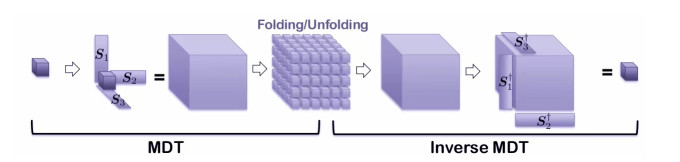
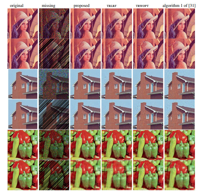
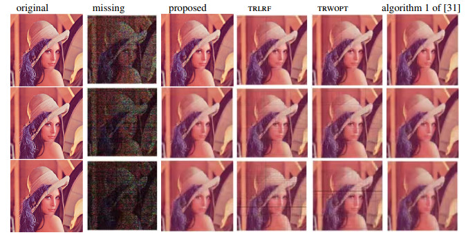
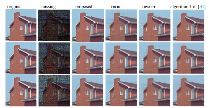
In this paper, we put up with a new algorithm for tensor completion problems that include missing slices or row/column fibers, where embedding a structured tensor by a multi-way delay-embedding transform (MDT) makes the tensor to be completed have a special structure. The main idea is to employ a tensor completion algorithm based on the tensor ring rank, constructing latent tensor ring factors with a structure that approximates the original tensor starting from the tensor structure. It is also proved that the sequence generated by the new algorithm converges to the optimal solution. Finally, the feasibility of the proposed algorithm is verified by experiments. Compared with other completed algorithms based on tensor ring rank, the completed accuracy is improved, up to 30%.

Keywords:

Citation: Ruiping Wen, Tingyan Liu, Yalei Pei. A new algorithm by embedding structured data for low-rank tensor ring completion[J]. AIMS Mathematics, 2025, 10(3): 6492-6511. doi: 10.3934/math.2025297

Related Papers:

[1]	Takao Komatsu, Ram Krishna Pandey . On hypergeometric Cauchy numbers of higher grade. AIMS Mathematics, 2021, 6(7): 6630-6646. doi: 10.3934/math.2021390
[2]	Takao Komatsu, Huilin Zhu . Hypergeometric Euler numbers. AIMS Mathematics, 2020, 5(2): 1284-1303. doi: 10.3934/math.2020088
[3]	Nadia N. Li, Wenchang Chu . Explicit formulae for Bernoulli numbers. AIMS Mathematics, 2024, 9(10): 28170-28194. doi: 10.3934/math.20241366
[4]	Taekyun Kim, Hye Kyung Kim, Dae San Kim . Some identities on degenerate hyperbolic functions arising from $p$ -adic integrals on $\mathbb{Z}_p$ . AIMS Mathematics, 2023, 8(11): 25443-25453. doi: 10.3934/math.20231298
[5]	Jizhen Yang, Yunpeng Wang . Congruences involving generalized Catalan numbers and Bernoulli numbers. AIMS Mathematics, 2023, 8(10): 24331-24344. doi: 10.3934/math.20231240
[6]	Taekyun Kim, Dae San Kim, Jin-Woo Park . Degenerate $r$ -truncated Stirling numbers. AIMS Mathematics, 2023, 8(11): 25957-25965. doi: 10.3934/math.20231322
[7]	Dojin Kim, Patcharee Wongsason, Jongkyum Kwon . Type 2 degenerate modified poly-Bernoulli polynomials arising from the degenerate poly-exponential functions. AIMS Mathematics, 2022, 7(6): 9716-9730. doi: 10.3934/math.2022541
[8]	Aimin Xu . Some identities connecting Stirling numbers, central factorial numbers and higher-order Bernoulli polynomials. AIMS Mathematics, 2025, 10(2): 3197-3206. doi: 10.3934/math.2025148
[9]	Waseem A. Khan, Abdulghani Muhyi, Rifaqat Ali, Khaled Ahmad Hassan Alzobydi, Manoj Singh, Praveen Agarwal . A new family of degenerate poly-Bernoulli polynomials of the second kind with its certain related properties. AIMS Mathematics, 2021, 6(11): 12680-12697. doi: 10.3934/math.2021731
[10]	Xhevat Z. Krasniqi . Approximation of functions in a certain Banach space by some generalized singular integrals. AIMS Mathematics, 2024, 9(2): 3386-3398. doi: 10.3934/math.2024166

Abstract

1. Introduction

L. Carlitz (^[1]) introduced analogues of Bernoulli numbers for the rational function (finite) field $K = \mathbb F_r(T)$ , which are called Bernoulli-Carlitz numbers now. Bernoulli-Carlitz numbers have been studied since then (e.g., see ^[2,3,4,5,6]). According to the notations by Goss ^[7], Bernoulli-Carlitz numbers $BC_n$ are defined by

$\begin{equation} \frac{x}{e_C(x)} = \sum\limits_{n = 0}^\infty\frac{BC_n}{\Pi(n)}x^n\,. \end{equation}$

(1.1)

Here, $e_C(x)$ is the Carlitz exponential defined by

$\begin{equation} e_C(x) = \sum\limits_{i = 0}^\infty\frac{x^{r^i}}{D_i}\,, \end{equation}$

(1.2)

where $D_i = [i][i-1]^r\cdots [1]^{r^{i-1}}$ ( $i\ge 1$ ) with $D_0 = 1$ , and $[i] = T^{r^i}-T$ . The Carlitz factorial $\Pi(i)$ is defined by

$\begin{equation} \Pi(i) = \prod\limits_{j = 0}^m D_j^{c_j} \end{equation}$

(1.3)

for a non-negative integer $i$ with $r$ -ary expansion:

$\begin{equation} i = \sum\limits_{j = 0}^m c_j r^j\quad (0\le c_j \lt r)\,. \end{equation}$

(1.4)

As analogues of the classical Cauchy numbers $c_n$ , Cauchy-Carlitz numbers $CC_n$ (^[8]) are introduced as

$\begin{equation} \frac{x}{\log_C(x)} = \sum\limits_{n = 0}^\infty\frac{CC_n}{\Pi(n)}x^n\,. \end{equation}$

(1.5)

Here, $\log_C(x)$ is the Carlitz logarithm defined by

$\begin{equation} \log_C(x) = \sum\limits_{i = 0}^\infty(-1)^i\frac{x^{r^i}}{L_i}\,, \end{equation}$

(1.6)

where $L_i = [i][i-1]\cdots [1]$ ( $i\ge 1$ ) with $L_0 = 1$ .

In ^[8], Bernoulli-Carlitz numbers and Cauchy-Carlitz numbers are expressed explicitly by using the Stirling-Carlitz numbers of the second kind and of the first kind, respectively. These properties are the extensions that Bernoulli numbers and Cauchy numbers are expressed explicitly by using the Stirling numbers of the second kind and of the first kind, respectively.

On the other hand, for $N\ge 1$ , hypergeometric Bernoulli numbers $B_{N, n}$ (^[9,10,11,12]) are defined by the generating function

$\begin{equation} \frac{1}{{}_1 F_1(1;N+1;x)} = \frac{x^N/N!}{e^x-\sum_{n = 0}^{N-1}x^n/n!} = \sum\limits_{n = 0}^\infty B_{N,n}\frac{x^n}{n!}\,, \end{equation}$

(1.7)

where

${}_1 F_1(a;b;z) = \sum\limits_{n = 0}^\infty\frac{(a)^{(n)}}{(b)^{(n)}}\frac{z^n}{n!}$

is the confluent hypergeometric function with $(x)^{(n)} = x(x+1)\cdots(x+n-1)$ ( $n\ge 1$ ) and $(x)^{(0)} = 1$ . When $N = 1$ , $B_n = B_{1, n}$ are classical Bernoulli numbers defined by

$\frac{x}{e^x-1} = \sum\limits_{n = 0}^\infty B_n\frac{x^n}{n!}\,.$

In addition, hypergeometric Cauchy numbers $c_{N, n}$ (see ^[13]) are defined by

$\begin{equation} \frac{1}{{}_2 F_1(1,N;N+1;-x)} = \frac{(-1)^{N-1}x^N/N}{\log(1+t)-\sum_{n = 1}^{N-1}(-1)^{n-1}x^n/n} = \sum\limits_{n = 0}^\infty c_{N,n}\frac{x^n}{n!}\,, \end{equation}$

(1.8)

where

${}_2 F_1(a,b;c;z) = \sum\limits_{n = 0}^\infty\frac{(a)^{(n)}(b)^{(n)}}{(c)^{(n)}}\frac{z^n}{n!}$

is the Gauss hypergeometric function. When $N = 1$ , $c_n = c_{1, n}$ are classical Cauchy numbers defined by

$\frac{x}{\log(1+x)} = \sum\limits_{n = 0}^\infty c_n\frac{x^n}{n!}\,.$

In ^[14], for $N\ge 0$ , the truncated Bernoulli-Carlitz numbers $BC_{N, n}$ and the truncated Cauchy-Carlitz numbers $CC_{N, n}$ are defined by

$\begin{equation} \frac{x^{r^N}/D_N}{e_C(x)-\sum_{i = 0}^{N-1}x^{r^i}/D_i} = \sum\limits_{n = 0}^\infty\frac{BC_{N,n}}{\Pi(n)}x^n \end{equation}$

(1.9)

and

$\begin{equation} \frac{(-1)^N x^{r^N}/L_N}{\log_C(x)-\sum_{i = 0}^{N-1}(-1)^i x^{r^i}/L_i} = \sum\limits_{n = 0}^\infty\frac{CC_{N,n}}{\Pi(n)}x^n\,, \end{equation}$

(1.10)

respectively. When $N = 0$ , $BC_n = BC_{0, n}$ and $CC_n = CC_{0, n}$ are the original Bernoulli-Carlitz numbers and Cauchy-Carlitz numbers, respectively. These numbers $BC_{N, n}$ and $CC_{N, n}$ in (1.9) and (1.10) in function fields are analogues of hypergeometric Bernoulli numbers in (1.7) and hypergeometric Cauchy numbers in (1.8) in complex numbers, respectively. In ^[15], the truncated Euler polynomials are introduced and studied in complex numbers.

It is known that any real number $\alpha$ can be expressed uniquely as the simple continued fraction expansion:

$\begin{equation} \alpha = a_0+\cfrac{1}{a_1+\cfrac{1}{a_2+\cfrac{1}{a_3+\ddots}}}\,, \end{equation}$

(1.11)

where $a_0$ is an integer and $a_1, a_2, \dots$ are positive integers. Though the expression is not unique, there exist general continued fraction expansions for real or complex numbers, and in general, analytic functions $f(x)$ :

$\begin{equation} f(x) = a_0(x)+\cfrac{b_1(x)}{a_1(x)+\cfrac{b_2(x)}{a_2(x)+\cfrac{b_3(x)}{a_3(x)+{\atop\ddots}}}}\,, \end{equation}$

(1.12)

where $a_0(x), a_1(x), \dots$ and $b_1(x), b_2(x), \dots$ are polynomials in $x$ . In ^[16,17] several continued fraction expansions for non-exponential Bernoulli numbers are given. For example,

$\begin{equation} \sum\limits_{n = 1}^\infty B_{2 n}(4 x)^n = \cfrac{x}{1+\dfrac{1}{2}+\cfrac{x}{\dfrac{1}{2}+\dfrac{1}{3}+\cfrac{x}{\dfrac{1}{3}+\dfrac{1}{4}+\cfrac{x}{\ddots}}}}\,. \end{equation}$

(1.13)

More general continued fractions expansions for analytic functions are recorded, for example, in ^[18]. In this paper, we shall give expressions for truncated Bernoulli-Carlitz numbers and truncated Cauchy-Carlitz numbers.

In ^[19], the hypergeometric Bernoulli numbers $B_{N, n}$ ( $N\ge 1$ , $n\ge 1$ ) can be expressed as

$B_{N,n} = (-1)^n n!\left| \begin{array}{ccccc} \frac{N!}{(N+1)!}&1&0&&\\ \frac{N!}{(N+2)!}&\frac{N!}{(N+1)!}&&&\\ \vdots&\vdots&\ddots&1&0\\ \frac{N!}{(N+n-1)!}&\frac{N!}{(N+n-2)!}&\cdots&\frac{N!}{(N+1)!}&1\\ \frac{N!}{(N+n)!}&\frac{N!}{(N+n-1)!}&\cdots&\frac{N!}{(N+2)!}&\frac{N!}{(N+1)!} \end{array} \right|\,.$

When $N = 1$ , we have a determinant expression of Bernoulli numbers ([,p.53]). In addition, relations between $B_{N, n}$ and $B_{N-1, n}$ are shown in ^[19].

In ^[21,22], the hypergeometric Cauchy numbers $c_{N, n}$ ( $N\ge 1$ , $n\ge 1$ ) can be expressed as

$c_{N,n} = n!\left| \begin{array}{ccccc} \frac{N}{N+1}&1&0&&\\ \frac{N}{N+2}&\frac{N}{N+1}&&&\\ \vdots&\vdots&\ddots&1&0\\ \frac{N}{N+n-1}&\frac{N}{N+n-2}&\cdots&\frac{N}{N+1}&1\\ \frac{N}{N+n}&\frac{N}{N+n-1}&\cdots&\frac{N}{N+2}&\frac{N}{N+1} \end{array} \right|\,.$

When $N = 1$ , we have a determinant expression of Cauchy numbers ([20,p.50]).

Recently, in (^[23]) the truncated Euler-Carlitz numbers $EC_{N, n}$ ( $N\ge 0$ ), introduced as

$\frac{x^{q^{2 N}}/D_{2 N}}{{\rm Cosh}_C(x)-\sum_{i = 0}^{N-1}x^{q^{2 i}}/D_{2 i}} = \sum\limits_{n = 0}^\infty\frac{EC_{N,n}}{\Pi(n)}x^n\,,$

are shown to have some determinant expressions. When $N = 0$ , $EC_n = EC_{0, n}$ are the Euler-Carlitz numbers, denoted by

$\frac{x}{{\rm Cosh}_C(x)} = \sum\limits_{n = 0}^\infty\frac{EC_{n}}{\Pi(n)}x^n\,,$

where

${\rm Cosh}_C(x) = \sum\limits_{i = 0}^\infty\frac{x^{q^{2 i}}}{D_{2 i}}$

is the Carlitz hyperbolic cosine. This reminds us that the hypergeometric Euler numbers $E_{N, n}$ (^[24]), defined by

$\frac{t^{2 N}/(2 N)!}{\cosh t-\sum_{n = 0}^{N-1}t^{2 n}/(2 n)!} = \sum\limits_{n = 0}^\infty E_{N,n}\frac{x^n}{n!}\,,$

have a determinant expression [,Theorem 2.3] for $N\ge 0$ and $n\ge 1$ ,

$E_{N, 2 n} = (-1)^n(2 n)! \left| \begin{array}{cccc} \frac{(2 N)!}{(2 N+2)!}&1&0&\\ \frac{(2 N)!}{(2 N+4)!}&\ddots&\ddots&0\\ \vdots&&\ddots&1\\ \frac{(2 N)!}{(2 N+2 n)!}&\cdots&\frac{(2 N)!}{(2 N+4)!}&\frac{(2 N)!}{(2 N+2)!} \end{array} \right|\,.$

When $N = 0$ , we have a determinant expression of Euler numbers (cf. [20,p.52]). More general cases are studied in ^[26].

In this paper, we also give similar determinant expressions of truncated Bernoulli-Carlitz numbers and truncated Cauchy-Carlitz numbers as natural extensions of those of hypergeometric numbers.

2. Continued fraction expansions of truncated Bernoulli-Carlitz and Cauchy-Carlitz numbers

Let the $n$ -th convergent of the continued fraction expansion of (1.12) be

$\begin{equation} \frac{P_n(x)}{Q_n(x)} = a_0(x)+\cfrac{b_1(x)}{a_1(x)+\cfrac{b_2(x)}{a_2(x)+{\atop\ddots{\atop+\cfrac{b_n(x)}{a_n(x)}}}}}\,. \end{equation}$

(2.1)

There exist the fundamental recurrence formulas:

$\begin{align} P_n(x)& = a_n(x)P_{n-1}(x)+b_n(x)P_{n-2}(x)\; (n\ge 1),\\ Q_n(x)& = a_n(x)Q_{n-1}(x)+b_n(x)Q_{n-2}(x)\; (n\ge 1), \end{align}$

(2.2)

with $P_{-1}(x) = 1$ , $Q_{-1}(x) = 0$ , $P_0(x) = a_0(x)$ and $Q_0(x) = 1$ .

From the definition in (1.9), truncated Bernoulli-Carlitz numbers satisfy the relation

$\left(D_N\sum\limits_{i = 0}^\infty\frac{x^{r^{N+i}-r^N}}{D_{N+i}}\right)\left(\sum\limits_{n = 0}^\infty\frac{BC_{N,n}}{\Pi(n)}x^n\right) = 1\,.$

Thus,

$P_m(x) = \frac{D_{N+m}}{D_N},\quad Q_m(x) = D_{N+m}\sum\limits_{i = 0}^m\frac{x^{r^{N+i}-r^N}}{D_{N+i}}$

yield that

$Q_m(x)\sum\limits_{n = 0}^\infty\frac{BC_{N,n}}{\Pi(n)}x^n\sim P_m(x)\quad(m\to\infty)\,.$

Notice that the $n$ -th convergent $p_n/q_n$ of the simple continued fraction (1.11) of a real number $\alpha$ yields the approximation property

$|q_n\alpha-p_n| \lt \frac{1}{q_{n+1}}\,.$

Now,

$\frac{P_0(x)}{Q_0(x)} = 1 = \frac{1}{1},\quad \frac{P_1(x)}{Q_1(x)} = 1-\frac{x^{r^{N+1}-r^N}}{D_{N+1}/D_N+x^{r^{N+1}-r^N}}$

and $P_n(x)$ and $Q_n(x)$ ( $n\ge 2$ ) satisfy the recurrence relations

$\begin{align*} P_n(x)& = \left(\frac{D_{N+n}}{D_{N+n-1}}+x^{r^{N+n}-r^{N+n-1}}\right)P_{n-1}(x)-\frac{D_{N+n-1}}{D_{N+n-2}}x^{r^{N+n}-r^{N+n-1}}P_{n-2}(x)\\ Q_n(x)& = \left(\frac{D_{N+n}}{D_{N+n-1}}+x^{r^{N+n}-r^{N+n-1}}\right)Q_{n-1}(x)-\frac{D_{N+n-1}}{D_{N+n-2}}x^{r^{N+n}-r^{N+n-1}}Q_{n-2}(x) \end{align*}$

(They are proved by induction). Since by (2.2) for $n\ge 2$

$a_n(x) = \frac{D_{N+n}}{D_{N+n-1}}+x^{r^{N+n}-r^{N+n-1}}\quad\hbox{and}\quad b_n(x) = -\frac{D_{N+n-1}}{D_{N+n-2}}x^{r^{N+n}-r^{N+n-1}}\,,$

we have the following continued fraction expansion.

Theorem 1.

$\sum\limits_{n = 0}^\infty\frac{BC_{N,n}}{\Pi(n)}x^n = 1-\cfrac{x^{r^{N+1}-r^N}}{\frac{D_{N+1}}{D_N}+x^{r^{N+1}-r^N}-\cfrac{\frac{D_{N+1}}{D_N}x^{r^{N+2}-r^{N+1}}}{\frac{D_{N+2}}{D_{N+1}}+x^{r^{N+2}-r^{N+1}}-\cfrac{\frac{D_{N+2}}{D_{N+1}}x^{r^{N+3}-r^{N+2}}}{\frac{D_{N+3}}{D_{N+2}}+x^{r^{N+3}-r^{N+2}}-{\atop\ddots}}}}\,.$

Put $N = 0$ in Theorem 1 to illustrate a simpler case. Then, we have a continued fraction expansion concerning the original Bernoulli-Carlitz numbers.

Corollary 1.

$\sum\limits_{n = 0}^\infty\frac{BC_{n}}{\Pi(n)}x^n = 1-\cfrac{x^{r-1}}{D_{1}+x^{r-1}-\cfrac{D_{1}x^{r^{2}-r}}{\frac{D_{2}}{D_{1}}+x^{r^{2}-r}-\cfrac{\frac{D_{2}}{D_{1}}x^{r^{3}-r^{2}}}{\frac{D_{3}}{D_{2}}+x^{r^{3}-r^{2}}-{\atop\ddots}}}}\,.$

From the definition in (1.10), truncated Cauchy-Carlitz numbers satisfy the relation

$\left(L_N\sum\limits_{i = 0}^\infty\frac{(-1)^i x^{r^{N+i}-r^N}}{L_{N+i}}\right)\left(\sum\limits_{n = 0}^\infty\frac{CC_{N,n}}{\Pi(n)}x^n\right) = 1\,.$

Thus,

$P_m(x) = \frac{L_{N+m}}{L_N},\quad Q_m(x) = L_{N+m}\sum\limits_{i = 0}^m\frac{(-1)^i x^{r^{N+i}-r^N}}{L_{N+i}}$

yield that

$Q_m(x)\sum\limits_{n = 0}^\infty\frac{CC_{N,n}}{\Pi(n)}x^n\sim P_m(x)\quad(m\to\infty)\,.$

Now,

$\frac{P_0(x)}{Q_0(x)} = 1 = \frac{1}{1},\quad \frac{P_1(x)}{Q_1(x)} = 1+\frac{x^{r^{N+1}-r^N}}{L_{N+1}/L_N-x^{r^{N+1}-r^N}}$

and $P_n(x)$ and $Q_n(x)$ ( $n\ge 2$ ) satisfy the recurrence relations

$\begin{align*} P_n(x)& = \left(\frac{L_{N+n}}{L_{N+n-1}}-x^{r^{N+n}-r^{N+n-1}}\right)P_{n-1}(x)+\frac{L_{N+n-1}}{L_{N+n-2}}x^{r^{N+n}-r^{N+n-1}}P_{n-2}(x)\\ Q_n(x)& = \left(\frac{L_{N+n}}{L_{N+n-1}}-x^{r^{N+n}-r^{N+n-1}}\right)Q_{n-1}(x)+\frac{L_{N+n-1}}{L_{N+n-2}}x^{r^{N+n}-r^{N+n-1}}Q_{n-2}(x)\,. \end{align*}$

Since by (2.2) for $n\ge 2$

$a_n(x) = \frac{L_{N+n}}{L_{N+n-1}}-x^{r^{N+n}+r^{N+n-1}}\quad\hbox{and}\quad b_n(x) = \frac{L_{N+n-1}}{L_{N+n-2}}x^{r^{N+n}-r^{N+n-1}}\,,$

we have the following continued fraction expansion.

Theorem 2.

$\sum\limits_{n = 0}^\infty\frac{CC_{N,n}}{\Pi(n)}x^n = 1+\cfrac{x^{r^{N+1}-r^N}}{\frac{L_{N+1}}{L_N}-x^{r^{N+1}-r^N}+\cfrac{\frac{L_{N+1}}{L_N}x^{r^{N+2}-r^{N+1}}}{\frac{L_{N+2}}{L_{N+1}}-x^{r^{N+2}-r^{N+1}}+\cfrac{\frac{L_{N+2}}{L_{N+1}}x^{r^{N+3}-r^{N+2}}}{\frac{L_{N+3}}{L_{N+2}}-x^{r^{N+3}-r^{N+2}}+{\atop\ddots}}}}\,.$

3. A determinant expression of truncated Cauchy-Carlitz numbers

In ^[14], some expressions of truncated Cauchy-Carlitz numbers have been shown. One of them is for integers $N\ge 0$ and $n\ge 1$ ,

$\begin{equation} CC_{N,n} = \Pi(n)\sum\limits_{k = 1}^{n}(-L_N)^k\sum\limits_{i_1,\dots,i_k\ge 1\atop r^{N+i_1}+\cdots+r^{N+i_k} = n+k r^N}\frac{(-1)^{i_1+\cdots+i_k}}{L_{N+i_1}\cdots L_{N+i_k}} \end{equation}$

(3.1)

[14,Theorem 2].

Now, we give a determinant expression of truncated Cauchy-Carlitz numbers.

Theorem 3. For integers $N\ge 0$ and $n\ge 1$ ,

$CC_{N,n} = \Pi(n)\left| \begin{array}{ccccc} -a_1&1&0&&\\ a_2&-a_1&\ddots&&\\ \vdots&&\ddots&\ddots&0\\ \vdots&&&-a_1&1\\ (-1)^n a_n&\cdots&\cdots&a_2&-a_1 \end{array} \right|\,,$

where

$a_l = \frac{(-1)^{i}L_N\delta_l^\ast}{L_{N+i}}\quad(l\ge 1)$

with

$\begin{equation} \delta_l^\ast = \begin{cases} 1&\mathit{\text{if $l = r^{N+i}-r^N\;(i = 0,1,\dots)$}};\\ 0&\mathit{\text{otherwise}}. \end{cases} \end{equation}$

(3.2)

We need the following Lemma in ^[27] in order to prove Theorem 3.

Lemma 1. Let $\{\alpha_n\}_{n\ge 0}$ be a sequence with $\alpha_0 = 1$ , and $R(j)$ be a function independent of $n$ . Then

$\begin{equation} \alpha_n = \left| \begin{array}{ccccc} R(1)&1&0&&\\ R(2)&R(1)&&&\\ \vdots&\vdots&\ddots&1&0\\ R(n-1)&R(n-2)&\cdots&R(1)&1\\ R(n)&R(n-1)&\cdots&R(2)&R(1) \end{array} \right|\,. \end{equation}$

(3.3)

if and only if

$\begin{equation} \alpha_n = \sum\limits_{j = 1}^n(-1)^{j-1}R(j)\alpha_{n-j}\quad(n\ge 1) \end{equation}$

(3.4)

with $\alpha_0 = 1$ .

Proof of Theorem 3. By the definition (1.10) with (1.6), we have

$\begin{align*} 1& = \left(\sum\limits_{i = 0}^\infty(-1)^i\frac{L_N}{L_{N+i}}\right)x^{r^{N+i}-r^N}\left(\sum\limits_{m = 0}^\infty\frac{CC_m}{\Pi(m)}x^m\right)\\ & = \left(\sum\limits_{l = 0}^\infty a_l x^l\right)\left(\sum\limits_{m = 0}^\infty\frac{CC_m}{\Pi(m)}x^m\right)\\ & = \sum\limits_{n = 0}^\infty\sum\limits_{l = 0}^\infty a_l\frac{CC_{n-l}}{\Pi(n-l)}x^n\,. \end{align*}$

Thus, for $n\ge 1$ , we get

$\sum\limits_{l = 0}^\infty a_l\frac{CC_{n-l}}{\Pi(n-l)} = 0\,.$

By Lemma 1, we have

$\begin{align*} \frac{CC_n}{\Pi(n)}& = -\sum\limits_{l = 1}^n a_l\frac{CC_{n-l}}{\Pi(n-l)}\\ & = \sum\limits_{l = 1}^n(-1)^{l-1}(-1)^l a_l\frac{CC_{n-l}}{\Pi(n-l)}\\ & = \left| \begin{array}{ccccc} -a_1&1&0&&\\ a_2&-a_1&\ddots&&\\ \vdots&&\ddots&\ddots&0\\ \vdots&&&-a_1&1\\ (-1)^n a_n&\cdots&\cdots&a_2&-a_1 \end{array} \right|\,. \end{align*}$

Examples. When $n = r^{N+1}-r^N$ ,

$\begin{align*} \frac{CC_{r^{N+1}-r^N}}{\Pi(r^{N+1}-r^N)}& = \left| \begin{array}{cccc} 0&1&&\\ \vdots&&\ddots&\\ 0&&&1\\ (-1)^{r^{N+1}-r^N}a_{r^{N+1}-r^N}&0&\cdots&0 \end{array}\right|\\ & = (-1)^{r^{N+1}-r^N+1}(-1)^{r^{N+1}-r^N}\frac{(-1)^{2 N+1}L_N}{L_{N+1}}\\ & = \frac{L_N}{L_{N+1}}\,. \end{align*}$

Let $n = r^{N+2}-r^N$ . For simplicity, put

$\begin{align*} \bar a& = (-1)^{r^{N+1}-r^N}(-1)^{2 N+1}\frac{L_N}{L_{N+1}}\,,\\ \hat a& = (-1)^{r^{N+2}-r^N}(-1)^{2 N+2}\frac{L_N}{L_{N+2}}\,. \end{align*}$

Then by expanding at the first column, we have

$\begin{align*} &\frac{CC_{r^{N+1}-r^N}}{\Pi(r^{N+1}-r^N)} = \left| \begin{array}{ccc} \underbrace{ \begin{array}{cccc} 0&1&0&\\ \vdots&&\ddots&\\ 0&&&\\ \bar a&&&\\ 0&\ddots&&\\ \vdots&&&\\ 0&&\ddots&\\ \hat a&0&\cdots&0 \end{array} }_{r^{N+2}-r^{N+1}} & \begin{array}{c} \\\\\\\\\\\\\\\\\bar a \end{array}& \underbrace{ \begin{array}{ccc} &&\\ &&\\ &&\\ &&\\ &&\\ &&\\ &\ddots&0\\ &&1\\ 0&\cdots&0 \end{array} }_{r^{N+1}-r^N-1} \end{array} \right|\\ & = (-1)^{r^{N+1}-r^N+1}\bar a\left| \begin{array}{cccc} \underbrace{ \begin{array}{ccc} 1&&\\ &\ddots&\\ &&1\\ \bar a&&\\ &\ddots&\\ &&\ddots\\ &&\\ && \end{array} }_{r^{N+1}-r^{N}-1} & \underbrace{ \begin{array}{cc} \\\\\\0&1\\&\ddots\\\\\\\\\ddots&\\&\bar a \end{array} }_2& \underbrace{ \begin{array}{ccc} &&\\ &&\\ &&\\ &&\\ &&\\ &&\\ &&\\ &\ddots&1\\ &\cdots&0 \end{array} }_{r^{N+1}-r^N-1} \end{array} \right|\\ &\quad +(-1)^{r^{N+2}-r^N+1}\hat a \left|\begin{array}{ccccccc} 1&0&&&&&\\ &\ddots&&&&&\\ &&&&&&\\ \bar a&&&&&&\\ &\ddots&&&&&\\ &&\ddots&&&\ddots&0\\ &&&\bar a&&&1 \end{array}\right|\,. \end{align*}$

The second term is equal to

$(-1)^{r^{N+2}-r^N+1}(-1)^{r^{N+2}-r^N}\frac{L_N}{L_{N+2}} = -\frac{L_N}{L_{N+2}}\,.$

The first term is

$\begin{align*} &(-1)^{r^{N+1}-r^N+1}\bar a\left| \begin{array}{ccc} \underbrace{ \begin{array}{ccc} 0&1&\\ &&\\ \bar a&&\\ &\ddots&\\ &&\ddots\\ && \end{array} }_{r^{N+2}-2 r^{N+1}+r^N} & \begin{array}{c} \\\\\\\\\\\\\bar a \end{array}& \underbrace{ \begin{array}{ccc} &&\\ &&\\ &&\\ &&\\ &&\\ &&1\\ &&0 \end{array} }_{r^{N+1}-r^N-1} \end{array} \right|\\ & = (-1)^{2(r^{N+1}-r^N+1)}\bar a^2 \left| \begin{array}{cccc} \underbrace{ \begin{array}{ccc} 1&&\\ &\ddots&\\ &&1\\ \bar a&&\\ &\ddots&\\ &&\ddots\\ &&\\ && \end{array} }_{r^{N+1}-r^{N}-1} & \underbrace{ \begin{array}{cc} \\\\\\0&1\\&\ddots\\\\\\\\\ddots&\\&\bar a \end{array} }_2& \underbrace{ \begin{array}{ccc} &&\\ &&\\ &&\\ &&\\ &&\\ &&\\ &&\\ &\ddots&1\\ &\cdots&0 \end{array} }_{r^{N+1}-r^N-1} \end{array} \right|\\ & = (-1)^{r(r^{N+1}-r^N+1)}\bar a^r \underbrace{ \left| \begin{array}{cccc} 0&1&&\\ \vdots&&\ddots&\\ 0&&&1\\ \bar a&0&\cdots&0 \end{array} \right| }_{r^{N+1}-r^N} \\ & = (-1)^{(r+1)(r^{N+1}-r^N+1)}\bar a^{r+1}\\ & = (-1)^{(r+1)(r^{N+1}-r^N+1)}(-1)^{(r^{N+1}-r^N)(r+1)}(-1)^{r+1}\frac{L_N^{r+1}}{L_{N+1}^{r+1}}\\ & = \frac{L_N^{r+1}}{L_{N+1}^{r+1}}\,. \end{align*}$

Therefore,

$\frac{CC_{r^{N+1}-r^N}}{\Pi(r^{N+1}-r^N)} = \frac{L_N^{r+1}}{L_{N+1}^{r+1}}-\frac{L_N}{L_{N+2}}\,.$

From this procedure, it is also clear that $CC_{N, n} = 0$ if $r^{N+1}-r^N\nmid n$ , since all the elements of one column (or row) become zero.

4. A determinant expression of truncated Bernoulli-Carlitz numbers

In ^[14], some expressions of truncated Bernoulli-Carlitz numbers have been shown. One of them is for integers $N\ge 0$ and $n\ge 1$ ,

$\begin{equation} BC_{N,n} = \Pi(n)\sum\limits_{k = 1}^{n}(-D_N)^k\sum\limits_{i_1,\dots,i_k\ge 1\atop r^{N+i_1}+\cdots+r^{N+i_k} = n+k r^N}\frac{1}{D_{N+i_1}\cdots D_{N+i_k}} \end{equation}$

(4.1)

[14,Theorem 1].

Now, we give a determinant expression of truncated Bernoulli-Carlitz numbers.

Theorem 4. For integers $N\ge 0$ and $n\ge 1$ ,

$BC_{N,n} = \Pi(n)\left| \begin{array}{ccccc} -d_1&1&0&&\\ d_2&-d_1&\ddots&&\\ \vdots&&\ddots&\ddots&0\\ \vdots&&&-d_1&1\\ (-1)^n d_n&\cdots&\cdots&d_2&-d_1 \end{array} \right|\,,$

where

$d_l = \frac{D_N\delta_l^\ast}{D_{N+i}}\quad(l\ge 1)$

with $\delta_l^\ast$ as in (3.2).

Proof. The proof is similar to that of Theorem 3, using (1.9) and (1.2).

Example. Let $n = 2(r^{N+1}-r^N)$ . For convenience, put

$\bar d = \frac{D_N}{D_{N+1}}\,.$

Then, we have

$\begin{align*} &\frac{BC_{N,2(r^{N+1}-r^N)}}{\Pi\bigl(2(r^{N+1}-r^N)\bigr)} = \left|\begin{array}{cc} \underbrace{ \begin{array}{ccc} 0&1&\\ \vdots&&\\ 0&&\\ \bar d&&\\ &\ddots&\\ &&\bar d \end{array} }_{r^{N+1}-r^N+1}& \underbrace{ \begin{array}{ccc} &&\\ &&\\ &&\\ &&\\ &&1\\ 0&\cdots&0 \end{array} }_{r^{N+1}-r^N-1} \end{array}\right|\\ & = (-1)^{r^{N+1}-r^N+1}\left| \begin{array}{ccc} \underbrace{ \begin{array}{ccc} 1&&\\ &\ddots&\\ &&1\\ \bar d&&\\ &\ddots&\\ &&\ddots\\ && \end{array} }_{r^{N+1}-r^N-1}& \begin{array}{c} \\\\\\0\\\\\\\\\bar d \end{array}& \underbrace{ \begin{array}{ccc} &&\\ &&\\ &&\\ 1&&\\ &\ddots&\\ &&1\\ &&0 \end{array} }_{r^{N+1}-r^N-1} \end{array} \right|\\ & = (-1)^{r^{N+1}-r^N+1}\bar d \underbrace{ \left| \begin{array}{cccc} 0&1&&\\ &&\ddots&\\ &&&1\\ \bar d&&&0 \end{array} \right| }_{r^{N+1}-r^N} \\ & = (-1)^{2(r^{N+1}-r^N+1)}\bar d^2 \left| \begin{array}{ccc} 1&&\\ &\ddots&\\ &&1 \end{array} \right|\\ & = \frac{D_N^2}{D_{N+1}^2}\,. \end{align*}$

It is also clear that $BC_{N, n} = 0$ if $r^{N+1}-r^N\nmid n$ .

5. Applications by the Trudi's formula

We shall use Trudi's formula to obtain different explicit expressions and inversion relations for the numbers $CC_{N, n}$ and $BC_{N, n}$ .

Lemma 2. For a positive integer $n$ , we have

$\left| \begin{array}{ccccc} a_1 & a_0 & 0 &\cdots & \\ a_2 & a_1 & \ddots & & \vdots \\ \vdots & \vdots & \ddots & \ddots & 0 \\ a_{n-1} & & \cdots &a_1 & a_0 \\ a_n & a_{n-1} & \cdots & a_2 & a_1 \end{array} \right| = \sum\limits_{t_1 + 2t_2 + \cdots +n t_n = n}\binom{t_1+\cdots + t_n}{t_1, \dots,t_n}(-a_0)^{n-t_1-\cdots - t_n}a_1^{t_1}a_2^{t_2}\cdots a_n^{t_n},$

where $\binom{t_1+\cdots + t_n}{t_1, \dots, t_n} = \frac{(t_1+\cdots + t_n)!}{t_1!\cdots t_n!}$ are the multinomial coefficients.

This relation is known as Trudi's formula [,Vol.3,p.214], ^[29] and the case $a_0 = 1$ of this formula is known as Brioschi's formula ^[30], [28,Vol.3,pp.208–209].

In addition, there exists the following inversion formula (see, e.g. ^[27]), which is based upon the relation

$\sum\limits_{k = 0}^n(-1)^{n-k}\alpha_k D(n-k) = 0\quad(n\ge 1)\,.$

Lemma 3. If $\{\alpha_n\}_{n\geq 0}$ is a sequence defined by $\alpha_0 = 1$ and

$\alpha_n = \begin{vmatrix} D(1) & 1 &0 & \\ D(2) & \ddots & \ddots &0 \\ \vdots & \ddots & \ddots & 1\\ D(n) & \cdots & D(2) & D(1) \\ \end{vmatrix}, \ \mathit{\text{then}} \ D(n) = \begin{vmatrix} \alpha_1 & 1 &0 & \\ \alpha_2 & \ddots & \ddots &0 \\ \vdots & \ddots & \ddots & 1\\ \alpha_n & \cdots & \alpha_2 & \alpha_1 \\ \end{vmatrix}\,.$

From Trudi's formula, it is possible to give the combinatorial expression

$\alpha_n = \sum\limits_{t_1+2t_2+\cdots +n t_n = n}\binom{t_1+\cdots+t_n}{t_1, \dots, t_n}(-1)^{n-t_1-\cdots - t_n}D(1)^{t_1}D(2)^{t_2}\cdots D(n)^{t_n}\,.$

By applying these lemmata to Theorem 3 and Theorem 4, we obtain an explicit expression for the truncated Cauchy-Carlitz numbers and the truncated Bernoulli-Carlitz numbers.

Theorem 5. For integers $N\ge 0$ and $n\ge 1$ , we have

$CC_{N,n} = \Pi(n)\sum\limits_{t_1+2 t_2+\cdots+n t_n = n}\binom{t_1+\cdots+t_n}{t_1,\dots,t_n} (-1)^{n-t_2-t_4-\cdots-t_{2\left\lfloor{n/2}\right\rfloor}}a_1^{t_1}\cdots a_n^{t_n}\,,$

where $a_n$ are given in Theorem 3.

Theorem 6. For integers $N\ge 0$ and $n\ge 1$ , we have

$BC_{N,n} = \Pi(n)\sum\limits_{t_1+2 t_2+\cdots+n t_n = n}\binom{t_1+\cdots+t_n}{t_1,\dots,t_n} (-1)^{n-t_2-t_4-\cdots-t_{2\left\lfloor{n/2}\right\rfloor}}d_1^{t_1}\cdots d_n^{t_n}\,,$

where $d_n$ are given in Theorem 4.

By applying the inversion relation in Lemma 3 to Theorem 3 and Theorem 4, we have the following.

Theorem 7. For integers $N\ge 0$ and $n\ge 1$ , we have

$a_n = (-1)^n\left|\begin{array}{ccccc} \frac{CC_{N,1}}{\Pi(1)}&1&0&&\\ \frac{CC_{N,2}}{\Pi(2)}&\frac{CC_{N,1}}{\Pi(1)}&&&\\ \vdots&\vdots&\ddots&1&0\\ \frac{CC_{N,n-1}}{\Pi(n-1)}&\frac{CC_{N,n-2}}{\Pi(n-2)}&\cdots&\frac{CC_{N,1}}{\Pi(1)}&1\\ \frac{CC_{N,n}}{\Pi(n)}&\frac{CC_{N,n-1}}{\Pi(n-1)}&\cdots&\frac{CC_{N,2}}{\Pi(2)}&\frac{CC_{N,1}}{\Pi(1)} \end{array}\right|\,,$

where $a_n$ is given in Theorem 3.

Theorem 8. For integers $N\ge 0$ and $n\ge 1$ , we have

$d_n = (-1)^n\left|\begin{array}{ccccc} \frac{BC_{N,1}}{\Pi(1)}&1&0&&\\ \frac{BC_{N,2}}{\Pi(2)}&\frac{BC_{N,1}}{\Pi(1)}&&&\\ \vdots&\vdots&\ddots&1&0\\ \frac{BC_{N,n-1}}{\Pi(n-1)}&\frac{BC_{N,n-2}}{\Pi(n-2)}&\cdots&\frac{BC_{N,1}}{\Pi(1)}&1\\ \frac{BC_{N,n}}{\Pi(n)}&\frac{BC_{N,n-1}}{\Pi(n-1)}&\cdots&\frac{BC_{N,2}}{\Pi(2)}&\frac{BC_{N,1}}{\Pi(1)} \end{array}\right|\,,$

where $d_n$ is given in Theorem 4.

Acknowledgments

We would like to thank the referees for their valuable comments.

Conflict of interest

The authors declare no conflict of interest.

References

[1]	A. E. Water, A. C. Sankaranarayanan, R. G. Baraniuk, SpaRCS: recovering low-rank and sparse matrices from compressive measurements, In: NIPS'11: Proceedings of the 25th international conference on neural information processing systems, 2011, 1089–1097.
[2]	M. Bertalmio, G. Sapiro, V. Caselles, C. Ballester, Image inpainting, In: SIGGRAPH '00: Proceedings of the 27th annual conference on computer graphics and interactive techniques, 2000,417–424. https://doi.org/10.1145/344779.344972
[3]	N. Komodakis, Image completion using global optimization, In: 2006 IEEE computer society conference on computer vision and pattern recognition (CVPR'06), IEEE, New York, NY, USA, 17–22 June 2006,442–452. https://doi.org/10.1109/CVPR.2006.141
[4]	M. Mørup, Applications of tensor (multiway array) factorizations and decompositions in data mining, WIRS Data Min. Knowl., 1 (2011), 24–40. https://doi.org/10.1002/widm.1 doi: 10.1002/widm.1
[5]	P. Comon, X. Luciani, A. L. F. de Almeida, Tensor decompositions, alternating least squares and other tales, J. Chemom., 23 (2009), 393–405. https://doi.org/10.1002/cem.1236 doi: 10.1002/cem.1236
[6]	Q. Q. Shi, J. M. Yin, J. J. Cai, A. Cichocki, T. Yokota, L. Chen, et al., Block Hankel tensor ARIMA for mnltiple short time series forecasting, Proceedings of the AAAI Conference on Artificial Intelligence, 34 (2020), 5758–5766. https://doi.org/10.1609/aaai.v34i04.6032 doi: 10.1609/aaai.v34i04.6032
[7]	M. Signoretto, R. Van de Plas, B. De Moor, J. A. K. Suykens, Tensor versus matrix completion: a comparison with application to spectral data, IEEE Signal Process. Lett., 18 (2011), 403–406. https://doi.org/10.1109/LSP.2011.2151856 doi: 10.1109/LSP.2011.2151856
[8]	J. Liu, P. Musialski, P. Wonka, J. P. Ye, Tensor completion for estimating missing values in visual data, IEEE Trans. Pattern Anal. Mach. Intell., 35 (2013), 208–220. https://doi.org/10.1109/TPAMI.2012.39 doi: 10.1109/TPAMI.2012.39
[9]	F. L. Hitchcock, The expression of a tensor or a polyadic as a sum of products, Journal of Mathematics and Physics, 6 (1927), 164–189. https://doi.org/10.1002/sapm192761164 doi: 10.1002/sapm192761164
[10]	L. R. Tucker, R. F. Koopman, R. L. Linn, Evaluation of factor analytic research procedures by means of simulated correlation matrices, Psychometrika, 34 (1969), 421–459. https://doi.org/10.1007/BF02290601 doi: 10.1007/BF02290601
[11]	I. V. Oseledets, Tensor-train decomposition, SIAM J. Sci. Comput., 33 (2011), 2295–2317. https://doi.org/10.1137/090752286 doi: 10.1137/090752286
[12]	Q. B. Zhao, G. X. Zhou, S. L. Xie, L. Q. Zhang, A. Cichocki, Tensor ring decomposition, arXiv: 1606.05535.
[13]	Y. Y. Xu, W. T. Yin, A block coordinate descent method for regularized multiconvex optimization with applications to nonnegative tensor factorization and completion, SIAM Journal Imaging Sci., 6 (2013), 1758–1789. https://doi.org/10.1137/120887795 doi: 10.1137/120887795
[14]	Y. Y. Liu, F. H. Shang, L. C. Jiao, J. Cheng, H. Cheng, Trace norm regularized candecomp/parafac decomposition with missing data, IEEE Trans. Cybernetics, 45 (2015), 2437–2448. https://doi.org/10.1109/TCYB.2014.2374695 doi: 10.1109/TCYB.2014.2374695
[15]	J. A. Bengua, H. N. Phien, H. D. Tuan, M. N. Do, Efficient tensor completion for color image and video recovery: low-rank tensor train, IEEE Trans. Image Process., 26 (2017), 2466–2479. https://doi.org/10.1109/TIP.2017.2672439 doi: 10.1109/TIP.2017.2672439
[16]	Z. M. Zhang, S. Aeron, Exact tensor completion using t-svd, IEEE Trans. Signal Process., 65 (2017), 1511–1526. https://doi.org/10.1109/TSP.2016.2639466 doi: 10.1109/TSP.2016.2639466
[17]	Q. B. Zhao, L. Q. Zhang, A. Cichocki, Bayesian CP factorization of incomplete tensors with automatic rank determination, IEEE Trans. Pattern Anal. Mach. Intell., 37 (2015), 1751–1763. https://doi.org/10.1109/tpami.2015.2392756 doi: 10.1109/tpami.2015.2392756
[18]	X. Y. Chen, Z. C. He, L. J. Sun, A Bayesian tensor decomposition approach for spatiotemporal traffic data imputation, Transport. Res. C: Emer., 98 (2019), 73–84. https://doi.org/10.1016/j.trc.2018.11.003 doi: 10.1016/j.trc.2018.11.003
[19]	Z. Long, C. Zhu, J. N. Liu, Y. P. Liu, Bayesian low rank tensor ring for image recovery, IEEE Trans. Image Process., 30 (2021), 3568–3580. https://doi.org/10.1109/TIP.2021.3062195 doi: 10.1109/TIP.2021.3062195
[20]	L. H. Yuan, J. T. Cao, X. Y. Zhao, Q. Wu, Q. B. Zhao, Higher-dimension tensor completion via low-rank tensor ring decomposition, In: 2018 Asia-Pacific signal and information processing association annual summit and conference (APSIPA ASC), IEEE, Honolulu, HI, USA, 12–15 November 2018, 1071–1076. https://doi.org/10.23919/APSIPA.2018.8659708
[21]	Q. B. Zhao, M. Sugiyama, L. H. Yuan, A. Cichocki, Learning efficient tensor representations with ring-structured networks, In: ICASSP 2019 - 2019 IEEE international conference on acoustics, speech and signal processing (ICASSP), Brighton, UK, 12–17 May 2019, 8608–8612. https://doi.org/10.1109/ICASSP.2019.8682231
[22]	J. Z. Xue, Y. Q. Zhao, S. G. Huang, W. Z. Liao, J. C.-W. Chan, S. G. Kong, Multilayer sparsity-based tensor decomposition for low-rank tensor completion, IEEE Trans. Neur. Net. Learn. Syst., 33 (2022), 6916–6930. https://doi.org/10.1109/tnnls.2021.3083931 doi: 10.1109/tnnls.2021.3083931
[23]	J. Z. Xue, Y. Q. Zhao, Y. Y. Bu, J. C.-W. Chan, S. G. Kong, When Laplacian scale mixture meets three-layer transform: a parametric tensor sparsity for tensor completion, IEEE Trans. Cybernetics, 52 (2022), 13887–13901. https://doi.org/10.1109/TCYB.2021.3140148 doi: 10.1109/TCYB.2021.3140148
[24]	J. Z. Xue, Y.-Q. Zhao, T. L. Wu, J. C.-W. Chan, Tensor convolution-like low-rank dictionary for high-dimensional image representatio, IEEE Trans. Circ. Syst. Vid., 34 (2024), 13257–13270. https://doi.org/10.1109/TCSVT.2024.3442295 doi: 10.1109/TCSVT.2024.3442295
[25]	T. Ding, M. Sznaier, O. I. Camps, A rank minimization approach to video inpainting, In: 2007 IEEE 11th international conference on computer vision, IEEE, Riode Janeiro, Brazil, October 2007, 1–8. https://doi.org/10.1109/ICCV.2007.4408932
[26]	E. N. Lorenz, Deterministic nonperiodic flow, J. Atmos. Sci., 20 (1963), 130–141. https://doi.org/10.1175/1520-0469(1963)020<0130:DNF>2.0.CO; 2 doi: 10.1175/1520-0469(1963)020<0130:DNF>2.0.CO; 2
[27]	I. Markovsky, Structured low-rank approximation and its applications, Automatica, 44 (2008), 891–909. https://doi.org/10.1016/j.automatica.2007.09.011 doi: 10.1016/j.automatica.2007.09.011
[28]	P. Van Overschee, B. De Moor, Subspace algorithms for the stochastic identification problem, In: [1991] Proceedings of the 30th IEEE conference on decision and control, IEEE, Brighton, UK, 11–13 December 1991, 1321–1326. https://doi.org/10.1109/CDC.1991.261604
[29]	Y. Li, K. J. R. Liu, J. Razavilar, A parameter estimation scheme for damped sinusoidal signals based on low-rank Hankel approximation, IEEE Trans. Signal Process., 45 (1997), 481–486. https://doi.org/10.1109/78.554314 doi: 10.1109/78.554314
[30]	W. Q. Wang, V. Aggarwal, S. Aeron, Efficient low rank tensor ring completion, In: 2017 IEEE international conference on computer vision (ICCV), IEEE, Venice, Italy, 22–29 October 2017, 5698–5706. https://doi.org/10.1109/ICCV.2017.607
[31]	T. Yokota, B. Erem, S. Guler, S. K. Warfield, H. Hontani, Missing slice recovery for tensors using a low-rank model in embedded space, In: 2018 IEEE/CVF conference on computer vision and pattern recognition, IEEE, Salt Lake City, UT, USA, 18–23 June 2018, 8251–8259. https://doi.org/10.1109/CVPR.2018.00861
[32]	Y. Li, K. J. R. Liu, J. RazavilarK, A parameter estimation scheme for damped sinusoidal signals based on low-rank Hankel approximation, IEEE Trans. Signal Process., 45 (1997), 481–486. https://doi.org/10.1109/78.554314 doi: 10.1109/78.554314
[33]	T. G. Kolda, B. W. Bader, Tensor decompositions and applications, SIAM Rev., 51 (2009), 455–500. https://doi.org/10.1137/07070111X doi: 10.1137/07070111X
[34]	G. H. Golub, C. F. Van Loan, Matrix computations, 4 Eds., Johns Hopkins University Press, 2014.
[35]	J. F. Cai, E. J. Candès, Z. W. Shen, A singular value thresholding algorithm for matrix completion, SIAM J. Ooptimiz., 20 (2010), 1956–1982. https://doi.org/10.1137/080738970 doi: 10.1137/080738970
[36]	C. J. Hillar, L.-H. Lim, Most tensor problems are NP-hard, J. ACM, 60 (2013), 45. https://doi.org/10.1145/2512329 doi: 10.1145/2512329
[37]	M. Signoretto, Q. T. Dinh, L. De Lathauwer, J. A. K. Suykens, Learning with tensors: a framework based on convex optimization and spectral regularization, Mach. Learn., 94 (2014), 303–351. https://doi.org/10.1007/s10994-013-5366-3 doi: 10.1007/s10994-013-5366-3
[38]	L. H. Yuan, C. Li, D. Mandic, J. T. Cao, Q. B. Zhao, Tensor ring decomposition with rank minimization on latent space: an efficient approach for tensor completion, Proceedings of the AAAI Conference on Artificial Intelligence, 33 (2019), 9151–9158. https://doi.org/10.1609/aaai.v33i01.33019151 doi: 10.1609/aaai.v33i01.33019151
[39]	Z. C. Lin, M. M. Chen, Y. Ma, The augmented Lagrange multiplier method for exact recovery of corrupted low-rank matrices, arXiv: 1009.5055.
[40]	Z. Wang, A. C. Bovik, H. R. Sheikh, E. P. Simoncelli, Image quality assessment: from error visibility to structural similarity, IEEE Trans. Image Process., 13 (2004), 600–612. https://doi.org/10.1109/TIP.2003.819861 doi: 10.1109/TIP.2003.819861

Reader Comments

Your name:*

Email:*
© 2025 the Author(s), licensee AIMS Press. This is an open access article distributed under the terms of the Creative Commons Attribution License (http://creativecommons.org/licenses/by/4.0)