A discrete logistic model with conditional Hyers–Ulam stability

Douglas R. Anderson; Masakazu Onitsuka; Douglas R. Anderson; Masakazu Onitsuka

doi:10.3934/math.2025298

AIMS Mathematics

2025, Volume 10, Issue 3: 6512-6545. doi: 10.3934/math.2025298

Previous Article Next Article

Research article Special Issues

A discrete logistic model with conditional Hyers–Ulam stability

Douglas R. Anderson ¹,
Masakazu Onitsuka ^{2
,
,}

1.
Department of Mathematics, Concordia College, Moorhead, MN 56562, USA
2.
Department of Applied Mathematics, Okayama University of Science, Okayama 700-0005, Japan

Received: 16 December 2024 Revised: 17 March 2025 Accepted: 19 March 2025 Published: 24 March 2025
MSC : 39A30, 39A60

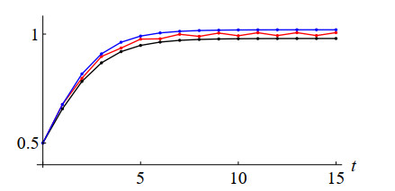
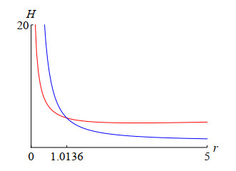
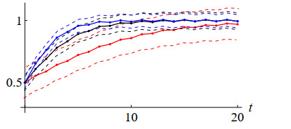
This study investigates the conditional Hyers–Ulam stability of a first-order nonlinear $ h $-difference equation, specifically a discrete logistic model. Identifying bounds on both the relative size of the perturbation and the initial population size is an important issue for nonlinear Hyers–Ulam stability analysis. Utilizing a novel approach, we derive explicit expressions for the optimal lower bound of the initial value region and the upper bound of the perturbation amplitude, surpassing the precision of previous research. Furthermore, we obtain a sharper Hyers–Ulam stability constant, which quantifies the error between true and approximate solutions, thereby demonstrating enhanced stability. The Hyers–Ulam stability constant is proven to be in terms of the step-size $ h $ and the growth rate but independent of the carrying capacity. Detailed examples are provided illustrating the applicability and sharpness of our results on conditional stability. In addition, a sensitivity analysis of the parameters appearing in the model is also performed.
- $ h $-difference equation,
- Hyers–Ulam stability,
- Hyers–Ulam stability constant,
- perturbation,
- conditional stability,
- logistic growth
Citation: Douglas R. Anderson, Masakazu Onitsuka. A discrete logistic model with conditional Hyers–Ulam stability[J]. AIMS Mathematics, 2025, 10(3): 6512-6545. doi: 10.3934/math.2025298

Related Papers:

Abstract

This study investigates the conditional Hyers–Ulam stability of a first-order nonlinear $ h $-difference equation, specifically a discrete logistic model. Identifying bounds on both the relative size of the perturbation and the initial population size is an important issue for nonlinear Hyers–Ulam stability analysis. Utilizing a novel approach, we derive explicit expressions for the optimal lower bound of the initial value region and the upper bound of the perturbation amplitude, surpassing the precision of previous research. Furthermore, we obtain a sharper Hyers–Ulam stability constant, which quantifies the error between true and approximate solutions, thereby demonstrating enhanced stability. The Hyers–Ulam stability constant is proven to be in terms of the step-size $ h $ and the growth rate but independent of the carrying capacity. Detailed examples are provided illustrating the applicability and sharpness of our results on conditional stability. In addition, a sensitivity analysis of the parameters appearing in the model is also performed.

References

[1]	J. Brzdęk, D. Popa, I. Raşa, B. Xu, Ulam stability of operators, Academic Press, 2018.
[2]	A. K. Tripathy, Hyers–Ulam stability of ordinary differential equations, Chapman and Hall/CRC, 2021. https://doi.org/10.1201/9781003120179
[3]	A. R. Baias, F. Blaga, D. Popa, On the best Ulam constant of a first order linear difference equation in Banach spaces, Acta Math. Hungar., 163 (2021), 563–575. https://doi.org/10.1007/s10474-020-01098-3 doi: 10.1007/s10474-020-01098-3
[4]	S. N. Bora, M. Shankar, Ulam–Hyers stability of second-order convergent finite difference scheme for first- and second-order nonhomogeneous linear differential equations with constant coefficients, Results Math., 78 (2023), 17. https://doi.org/10.1007/s00025-022-01791-5 doi: 10.1007/s00025-022-01791-5
[5]	K. Chen, Y. Si, Ulam type stability for the second-order linear Hahn difference equations, Appl. Math. Lett., 160 (2025), 109355. https://doi.org/10.1016/j.aml.2024.109355 doi: 10.1016/j.aml.2024.109355
[6]	D. M. Kerekes, B. Moşneguţu, D. Popa, On Ulam stability of a second order linear difference equation, AIMS Math., 8 (2023), 20254–20268. https://doi.org/10.3934/math.20231032 doi: 10.3934/math.20231032
[7]	A. Novac, D. Otrocol, D. Popa, Ulam stability of a linear difference equation in locally convex spaces, Results Math., 76 (2021), 33. https://doi.org/10.1007/s00025-021-01344-2 doi: 10.1007/s00025-021-01344-2
[8]	Y. Shen, Y. Li, The $z$-transform method for the Ulam stability of linear difference equations with constant coefficients, Adv. Differ. Equations, 2018 (2018), 396. https://doi.org/10.1186/s13662-018-1843-0 doi: 10.1186/s13662-018-1843-0
[9]	C. Buşe, V. Lupulescu, D. O'Regan, Hyers–Ulam stability for equations with differences and differential equations with time-dependent and periodic coefficients, Proc. R. Soc. Edinburgh Sect. A, 150 (2020), 2175–2188. https://doi.org/10.1017/prm.2019.12 doi: 10.1017/prm.2019.12
[10]	D. Popa, I. Raşa, A. Viorel, Approximate solutions of the logistic equation and Ulam stability, Appl. Math. Lett., 85 (2018), 64–69. https://doi.org/10.1016/j.aml.2018.05.018 doi: 10.1016/j.aml.2018.05.018
[11]	M. Onitsuka, Conditional Ulam stability and its application to the logistic model, Appl. Math. Lett., 122 (2021), 107565. https://doi.org/10.1016/j.aml.2021.107565 doi: 10.1016/j.aml.2021.107565
[12]	M. Onitsuka, Approximate solutions of generalized logistic equation, Discrete Contin. Dyn. Syst., 29 (2024), 4505–4526. https://doi.org/10.3934/dcdsb.2024053 doi: 10.3934/dcdsb.2024053
[13]	L. Backes, D. Dragičeviū, M. Onitsuka, M. Pituk, Conditional Lipschitz shadowing for ordinary differential equations, J. Dyn. Differ. Equations, 36 (2024), 3535–3552. https://doi.org/10.1007/s10884-023-10246-6 doi: 10.1007/s10884-023-10246-6
[14]	S. M. Jung, Y. W. Nam, Hyers–Ulam stability of Pielou logistic difference equation, J. Nonlinear Sci. Appl., 10 (2017), 3115–3122. https://doi.org/10.22436/jnsa.010.06.26 doi: 10.22436/jnsa.010.06.26
[15]	Y. W. Nam, Hyers–Ulam stability of elliptic Möbius difference equation, Cogent Math. Stat., 5 (2018), 1492338. https://doi.org/10.1080/25742558.2018.1492338 doi: 10.1080/25742558.2018.1492338
[16]	Y. W. Nam, Hyers–Ulam stability of hyperbolic Möbius difference equation, Filomat, 32 (2018), 4555–4575. https://doi.org/10.2298/fil1813555n doi: 10.2298/fil1813555n
[17]	Y. W. Nam, Hyers–Ulam stability of loxodromic Möbius difference equation, Appl. Math. Comput., 356 (2019), 119–136. https://doi.org/10.1016/j.amc.2019.03.033 doi: 10.1016/j.amc.2019.03.033
[18]	A. S. Ackleh, Y. M. Dib, S. R. J. Jang, A three-stage discrete-time population model: continuous versus seasonal reproduction, J. Biol. Dyn., 1 (2007), 291–304. https://doi.org/10.1080/17513750701605440 doi: 10.1080/17513750701605440
[19]	L. L. Albu, Non-linear models: applications in economics, SSRN Electron. J., 2006. https://doi.org/10.2139/ssrn.1565345
[20]	M. Bohner, A. Peterson, Advances in dynamic equations on time scales, Birkhäuser, 2003. https://doi.org/10.1007/978-0-8176-8230-9
[21]	J. Cushing, S. Henson, A periodically forced Beverton–Holt equation, J. Differ. Equations Appl., 8 (2002), 1119–1120. https://doi.org/10.1080/1023619031000081159 doi: 10.1080/1023619031000081159
[22]	S. Elaydi, R. J. Sacker, Global stability of periodic orbits of non-autonomous difference equations and population biology, J. Differ. Equations, 208 (2005), 258–273. https://doi.org/10.1016/j.jde.2003.10.024 doi: 10.1016/j.jde.2003.10.024
[23]	M. Bohner, A. Peterson, Dynamic equations on time scales: an introduction with applications, Birkhäuser, 2001. https://doi.org/10.1007/978-1-4612-0201-1

Reader Comments

Your name:*

Email:*
© 2025 the Author(s), licensee AIMS Press. This is an open access article distributed under the terms of the Creative Commons Attribution License (http://creativecommons.org/licenses/by/4.0)