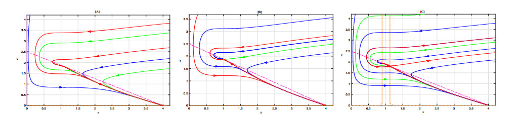
A nonsmooth ecological model was proposed and analyzed, focusing on IPM, state-dependent feedback control strategies, and anti-predator behavior. The main objective was to investigate the impact of anti-predator behavior on successful pest control, pest outbreaks, and the dynamical properties of the proposed model. First, the qualitative behaviors of the corresponding ODE model were presented, along with an accurate definition of the Poincaré map in the absence of internal equilibrium. Second, we investigated the existence and stability of order-k (where k = 1, 2, 3) periodic solutions through the monotonicity and continuity properties of the Poincaré map. Third, we conducted numerical simulations to investigate the complexity of the dynamical behaviors. Finally, we provided a precise definition of the Poincaré map in situations where an internal equilibrium existed within the model. The results indicated that when the mortality rate of the insecticide was low or high, the boundary order-1 periodic solution of the model was stable. However, when the mortality rate of the insecticide was maintained at a moderate level, the boundary order-1 periodic solution of the model became unstable; in this case, pests and natural enemies could coexist.
Citation: Shuai Chen, Wenjie Qin. Antipredator behavior of a nonsmooth ecological model with a state threshold control strategy[J]. AIMS Mathematics, 2024, 9(3): 7426-7448. doi: 10.3934/math.2024360
A nonsmooth ecological model was proposed and analyzed, focusing on IPM, state-dependent feedback control strategies, and anti-predator behavior. The main objective was to investigate the impact of anti-predator behavior on successful pest control, pest outbreaks, and the dynamical properties of the proposed model. First, the qualitative behaviors of the corresponding ODE model were presented, along with an accurate definition of the Poincaré map in the absence of internal equilibrium. Second, we investigated the existence and stability of order-k (where k = 1, 2, 3) periodic solutions through the monotonicity and continuity properties of the Poincaré map. Third, we conducted numerical simulations to investigate the complexity of the dynamical behaviors. Finally, we provided a precise definition of the Poincaré map in situations where an internal equilibrium existed within the model. The results indicated that when the mortality rate of the insecticide was low or high, the boundary order-1 periodic solution of the model was stable. However, when the mortality rate of the insecticide was maintained at a moderate level, the boundary order-1 periodic solution of the model became unstable; in this case, pests and natural enemies could coexist.

| [1] |
S. Kaul, On impulsive semidynamical systems, J. Math. Anal. Appl., 150 (1990), 120–128. https://doi.org/10.1016/0022-247X(90)90199-P doi: 10.1016/0022-247X(90)90199-P

|
| [2] |
Z. Cao, C. Li, X. Zhang, X. Yang, Robust exponential stabilization of stochastic coupled t-s fuzzy complex networks subject to state-dependent impulsive control, Int. J. Robust Nonlinear Control, 33 (2023), 3334–3357. https://doi.org/10.1002/rnc.6581 doi: 10.1002/rnc.6581
|
| [3] |
B. Tang, Y. Xiao, S. Tang, R. A. Cheke, A feedback control model of comprehensive therapy for treating immunogenic tumours, Int. J. Bifurcat. Chaos, 26 (2016), 1650039. https://doi.org/10.1142/S0218127416500395 doi: 10.1142/S0218127416500395
|
| [4] |
W. Qin, X. Tan, X. Shi, C. Xiang, IPM strategies to a discrete switching predator-prey model induced by a mate-finding allee effect, J. Biol. Dynam., 13 (2019), 586–605. https://doi.org/10.1080/17513758.2019.1682200 doi: 10.1080/17513758.2019.1682200
|
| [5] |
C. Bravo, M. Sarasa, V. Bretagnolle, O. Pays, Detectability and predator strategy affect egg depredation rates: Implications for mitigating nest depredation in farmlands, Sci. Total Environ., 829 (2022), 154558. https://doi.org/10.1016/j.scitotenv.2022.154558 doi: 10.1016/j.scitotenv.2022.154558
|
| [6] |
H. Liu, H. Cheng, Dynamic analysis of a prey–predator model with state-dependent control strategy and square root response function, Adv. Differ. Equ., 2018 (2018), 63. https://doi.org/10.1186/s13662-018-1507-0 doi: 10.1186/s13662-018-1507-0
|
| [7] |
Q. Zhang, S. Tang, Bifurcation analysis of an ecological model with nonlinear state-dependent feedback control by Poincaré map defined in phase set, Commun. Nonlinear Sci. Numer. Simul., 108 (2022), 106212. https://doi.org/10.1016/j.cnsns.2021.106212 doi: 10.1016/j.cnsns.2021.106212
|
| [8] | S. Tang, L. Chen, Modelling and analysis of integrated pest management strategy, Discrete Cont. Dynam. Syst. Ser. B, 4 (2004), 759–768. |
| [9] |
S. Tang, J. Liang, Y. Tan, R. A. Cheke, Threshold conditions for integrated pest management models with pesticides that have residual effects, J. Math. Biol., 66 (2013), 1–35. https://doi.org/10.1007/s00285-011-0501-x doi: 10.1007/s00285-011-0501-x
|
| [10] |
O. Akman, T. Comar, M. Henderson, An analysis of an impulsive stage structured integrated pest management model with refuge effect, Chaos Solit. Fract., 111 (2018), 44–54. https://doi.org/10.1016/j.chaos.2018.03.039 doi: 10.1016/j.chaos.2018.03.039
|
| [11] | S. K. Kaul, On impulsive semidynamical systems iii: Lyapunov stability, In: Recent Trends in Differential Equations, 1992,335–345. |
| [12] |
M. Huang, A. Yang, S. Yuan, T. Zhang, Stochastic sensitivity analysis and feedback control of noiseinduced transitions in a predator-prey model with anti-predator behavior, Math. Biosci. Eng., 20 (2023), 4219–4242. http://dx.doi.org/10.3934/mbe.2023197 doi: 10.3934/mbe.2023197
|
| [13] |
X. Wang, C. Huang, Y. Liu, A vertically transmitted epidemic model with two state-dependent pulse controls, Math. Biosci. Eng., 19 (2022), 13967–13987. http://dx.doi.org/10.3934/mbe.2022651 doi: 10.3934/mbe.2022651
|
| [14] |
T. Summers, E. King, D. Martin, R. Jackson, Biological control of diatraea saccharalis [lep.: Pyralidae] in florida by periodic releases of lixophaga diatraeae [dipt.: Tachinidae], Entomophaga, 21 (1976), 359–366. https://doi.org/10.1007/BF02371634 doi: 10.1007/BF02371634
|
| [15] |
S. Tang, Y. Xiao, L. Chen, R. A. Cheke, Integrated pest management models and their dynamical behaviour, Bull. Math. Biol., 67 (2005), 115–135. https://doi.org/10.1016/j.bulm.2004.06.005 doi: 10.1016/j.bulm.2004.06.005
|
| [16] |
S. Tang, W. Pang, On the continuity of the function describing the times of meeting impulsive set and its application, Math. Biosci. Eng., 14 (2017), 1399–1406. https://doi.org/10.3934/mbe.2017072 doi: 10.3934/mbe.2017072
|
| [17] |
S. Tang, X. Tan, J. Yang, J. Liang, Periodic solution bifurcation and spiking dynamics of impacting predator-prey dynamical model, Int. J. Bifurc. Chaos, 28 (2018), 1850147. https://doi.org/10.1142/S021812741850147X doi: 10.1142/S021812741850147X
|
| [18] |
Y. Tian, Y. Gao, K. Sun, A fishery predator-prey model with anti-predator behavior and complex dynamics induced by weighted fishing strategies, Math. Biosci. Eng., 20 (2023), 1558–1579. http://dx.doi.org/10.3934/mbe.2023071 doi: 10.3934/mbe.2023071
|
| [19] | Y. F. Li, C. Z. Zhu, Y. W. Liu, Dynamic analysis of a predator-prey model with state-dependent impulsive effects, Chinese Quart. J. Math., 38 (2023), 1. |
| [20] |
A. Janssen, F. Faraji, T. Van Der Hammen, S. Magalhaes, M. W. Sabelis, Interspecific infanticide deters predators, Ecology Lett., 5 (2002), 490–494. https://doi.org/10.1046/j.1461-0248.2002.00349.x doi: 10.1046/j.1461-0248.2002.00349.x
|
| [21] |
Y. Saito, Prey kills predator: Counter-attack success of a spider mite against its specific phytoseiid predator, Exp. Appl. Acarol., 2 (1986), 47–62. https://doi.org/10.1007/BF01193354 doi: 10.1007/BF01193354
|
| [22] |
F. Sanchez-Garduno, P. Miramontes, T. T. Marquez-Lago, Role reversal in a predator-prey interaction, Royal Soc. Open Sci., 1 (2014), 140186. https://doi.org/10.1098/rsos.140186 doi: 10.1098/rsos.140186
|
| [23] |
F. Faraji, A. Janssen, M. W. Sabelis, The benefits of clustering eggs: The role of egg predation and larval cannibalism in a predatory mite, Oecologia, 131 (2002), 20–26. https://doi.org/10.1007/s00442-001-0846-8 doi: 10.1007/s00442-001-0846-8
|
| [24] |
J. C. Van Lenteren, The state of commercial augmentative biological control: Plenty of natural enemies, but a frustrating lack of uptake, BioControl, 57 (2012), 1–20. https://doi.org/10.1007/s10526-011-9395-1 doi: 10.1007/s10526-011-9395-1
|
| [25] |
A. Janssen, E. Willemse, T. Van Der Hammen, Poor host plant quality causes omnivore to consume predator eggs, J. Animal Ecol., 72 (2003), 478–483. https://doi.org/10.1046/j.1365-2656.2003.00717.x doi: 10.1046/j.1365-2656.2003.00717.x
|
| [26] | R. A. Relyea, How prey respond to combined predators: A review and an empirical test, Ecology, 84 (2003), 1827–1839. https://doi.org/10.1890/0012-9658(2003)084[1827:HPRTCP]2.0.CO;2 |
| [27] |
Pallini, Janssen, Sabelis, Predators induce interspecific herbivore competition for food in refuge space, Ecol. Lett., 1 (1998), 171–177. https://doi.org/10.1046/j.1461-0248.1998.00019.x doi: 10.1046/j.1461-0248.1998.00019.x
|
| [28] |
Y. Tian, S. Tang, R. A. Cheke, Nonlinear state-dependent feedback control of a pest-natural enemy system, Nonlinear Dyn., 94 (2018), 2243–2263. https://doi.org/10.1007/s11071-018-4487-4 doi: 10.1007/s11071-018-4487-4
|
| [29] |
J. Yang, S. Tang, Holling type ii predator-prey model with nonlinear pulse as state-dependent feedback control, J. Comput. Appl. Math., 291 (2016), 225–241. https://doi.org/10.1016/j.cam.2015.01.017 doi: 10.1016/j.cam.2015.01.017
|
| [30] |
B. Tang, Y. Xiao, Bifurcation analysis of a predator-prey model with anti-predator behaviour, Chaos Solit. Fract., 70 (2015), 58–68. https://doi.org/10.1016/j.chaos.2014.11.008 doi: 10.1016/j.chaos.2014.11.008
|
| [31] |
C. Xiang, Z. Xiang, S. Tang, J. Wu, Discrete switching host-parasitoid models with integrated pest control, Int. J. Bifurcat. Chaos, 24 (2014), 1450114. https://doi.org/10.1142/S0218127414501144 doi: 10.1142/S0218127414501144
|


Figures(8) / Tables(2)

Shuai Chen, Wenjie Qin. Antipredator behavior of a nonsmooth ecological model with a state threshold control strategy[J]. AIMS Mathematics, 2024, 9(3): 7426-7448. doi: 10.3934/math.2024360


 DownLoad: