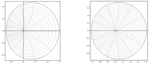
In the present paper, we investigated some conditions to be in the class of Carathéodory functions by using the concept of the first-order differential subordinations. Moreover, various interesting special cases were considered in the geometric function theory as applications of main results presented here.
Citation: Inhwa Kim, Young Jae Sim, Nak Eun Cho. First-order differential subordinations associated with Carathéodory functions[J]. AIMS Mathematics, 2024, 9(3): 5466-5479. doi: 10.3934/math.2024264
In the present paper, we investigated some conditions to be in the class of Carathéodory functions by using the concept of the first-order differential subordinations. Moreover, various interesting special cases were considered in the geometric function theory as applications of main results presented here.

| [1] |
D. A. Brannan, W. E. Kirwan, On some classes of bounded univalent functions, J. Lond. Math. Soc., s2-1 (1969), 431–443. https://doi.org/10.1112/jlms/s2-1.1.431 doi: 10.1112/jlms/s2-1.1.431

|
| [2] | C. Carathéodory, Über den variabilitätsbereich der coeffizienten von potenzreihen, die gegebene werte nicht annehmen, Math. Ann., 64 (1907), 95–115. |
| [3] | C. Carathéodory, Über den variabilitätsbereich der fourier'schen konstanten von positiven harmonischen funktionen, Rend. Circ. Mat. Palermo, 32 (1911), 193–217. |
| [4] | P. J. Eenigenburg, S. S. Miller, P. T. Mocanu, M. O. Reade, On a Briot-Bouquet differential subordination, General Inequalities 3, International Series of Numerical Mathematics, Basel: Birkh$\ddot{a}$user, 1983,339–348. |
| [5] | I. H. Kim, N. E. Cho, Sufficient conditions for Carathéodory functions, Comput. Math. Appl., 59 (2010), 2067–2073. |
| [6] | O. S. Kwon, Y. J. Sim, Sufficient conditions for Carathéodory functions and applications to univalent functions, Math. Slovaca, 69 (2019), 1065–1076. |
| [7] | M. S. Liu, Y. C. Zhu, Criteria for strongly starlike and $\Phi$-like functions, Complex Var. Elliptic Equ., 53 (2008), 485–500. |
| [8] |
S. S. Miller, P. T. Mocanu, Univalent solutions of Briot-Bouquet differential equations, J. Differ. Equ., 56 (1985), 297–309. https://doi.org/10.1016/0022-0396(85)90082-8 doi: 10.1016/0022-0396(85)90082-8
|
| [9] | S. S. Miller, P. T. Mocanu, Mark-Strohh$\ddot{a}$cker differential subordination systems, Proc. Amer. Math. Soc., 99 (1987), 527–534. |
| [10] | S. S. Miller, P. T. Mocanu, On some classes of first-order differential subordinations, Michigan Math. J., 32 (1985), 185–195. |
| [11] | S. S. Miller, P. T. Mocanu, A special differential subordination and its application to univalency conditions, Current Topics in Analytic Function Theory, Singapore, London: World Scientific, 1992,171–185. |
| [12] |
S. S. Miller, P. T. Mocanu, Briot-Bouquet differential equations and differential subordinations, Complex Var. Theory Appl.: Int. J., 33 (1997), 217–237. https://doi.org/10.1080/17476939708815024 doi: 10.1080/17476939708815024
|
| [13] | S. S. Miller, P. T. Mocanu, Differential Subordinations: Theory and Applications, New York, Basel: Marcel Dekker, 2000. |
| [14] | P. T. Mocanu, Alpha-convex integral operators and strongly starlike functions, Studia Univ. Babes-Bolyai Math., 34 (1989), 18–24. |
| [15] |
M. Nunokawa, On the order of strongly starlikeness of strongly convex functions, Proc. Japan Acad. Ser. A Math. Sci., 69 (1993), 234–237. https://doi.org/10.3792/pjaa.69.234 doi: 10.3792/pjaa.69.234
|
| [16] | M. Nunokawa, O. S. Kwon, Y. J. Sim, N. E. Cho, Sufficient conditions for Carathéodory functions, Filomat, 32 (2018), 1097–1106. |
| [17] |
M. S. Robertson, On the theory of univalent functions, Ann. Math., 37 (1936), 374–408. https://doi.org/10.2307/1968451 doi: 10.2307/1968451
|
| [18] | Y. J. Sim, O. S. Kwon, N. E. Cho, H. M. Srivastava, Some sets of sufficient conditions for Carathéodory functions, J. Comput. Anal. Appl., 21 (2016), 1243–1254. |
| [19] | R. Singh, On Bazilevć functions, Proc. Amer. Math. Soc., 38 (1973), 261–271. |
| [20] | J. Stankiewicz, Quelques problèmes extrémaux dans les classes des fonctions $\alpha$-angularirement étoilées, Ann. Univ. Mariae Curie-Skłodowska Sect. A, 20 (1966), 59–75. |
| [21] | J. Stankiewicz, On a family of starlike functions, Ann. Univ. Mariae Curie-Skłodowska Sect. A, 22-24 (1968–1970), 175–181. |
| [22] |
L. M. Wang, The tilted Carathéodory class and its applications, J. Korean Math. Soc., 49 (2012), 671–686. http://doi.org/10.4134/JKMS.2012.49.4.671 doi: 10.4134/JKMS.2012.49.4.671
|
| [23] |
D. R. Wilken, J. Feng, A remark on convex and starlike functions, J. Lond. Math. Soc., s2-21 (1980), 287–290. https://doi.org/10.1112/jlms/s2-21.2.287 doi: 10.1112/jlms/s2-21.2.287
|
Figures(1)

Inhwa Kim, Young Jae Sim, Nak Eun Cho. First-order differential subordinations associated with Carathéodory functions[J]. AIMS Mathematics, 2024, 9(3): 5466-5479. doi: 10.3934/math.2024264


 DownLoad: