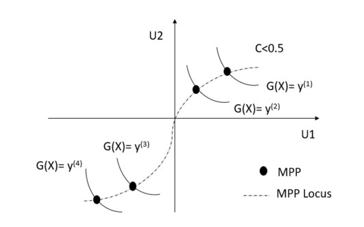
During the engineering structure's operation, the mechanical structure's performance and loading will change with time, so the parameter uncertainty and structural reliability will also have dynamic characteristics. The time-varying reliability analysis method can more accurately evaluate structural reliability by fully using this dynamic uncertainty. However, the time-varying reliability analysis was mainly based on the spanning rate method, which was complex and difficult to obtain the final result. Therefore, this study proposed an enhanced dung beetle optimization (EDBO) assisted time-varying reliability analysis method based on the adaptive Kriging model. With the help of the adaptive Kriging model and the EDBO optimization algorithm, the efficiency of the time-varying reliability analysis method was improved. At the same time, to prevent prematurely falling into the local search trap, the method improved the uniformity of the sample by initializing the sample through improved tent chaotic mapping (ITCM). Next, the Gaussian random walk strategy was used to search the updated position, which further improved the accuracy of the reliability analysis results. Finally, the accuracy and effectiveness of the proposed time-varying reliability analysis method were verified by four mechanical structure model examples. From the calculation results, it can be seen that with the help of the new DBO optimization algorithm, the relative error of the proposed reliability analysis results was about 20%~30% lower than that of the traditional reliability analysis method. What's more, the calculation efficiency was higher than that of other reliability analysis methods.
Citation: Yunhan Ling, Yiqing Shi, Huimin Hou, Lidong Pan, Hao Chen, Peixin Liang, Shiyuan Yang, Peng Nie, Jiahao Han, Debiao Meng. Enhanced dung beetle optimizer for Kriging-assisted time-varying reliability analysis[J]. AIMS Mathematics, 2024, 9(10): 29296-29332. doi: 10.3934/math.20241420
During the engineering structure's operation, the mechanical structure's performance and loading will change with time, so the parameter uncertainty and structural reliability will also have dynamic characteristics. The time-varying reliability analysis method can more accurately evaluate structural reliability by fully using this dynamic uncertainty. However, the time-varying reliability analysis was mainly based on the spanning rate method, which was complex and difficult to obtain the final result. Therefore, this study proposed an enhanced dung beetle optimization (EDBO) assisted time-varying reliability analysis method based on the adaptive Kriging model. With the help of the adaptive Kriging model and the EDBO optimization algorithm, the efficiency of the time-varying reliability analysis method was improved. At the same time, to prevent prematurely falling into the local search trap, the method improved the uniformity of the sample by initializing the sample through improved tent chaotic mapping (ITCM). Next, the Gaussian random walk strategy was used to search the updated position, which further improved the accuracy of the reliability analysis results. Finally, the accuracy and effectiveness of the proposed time-varying reliability analysis method were verified by four mechanical structure model examples. From the calculation results, it can be seen that with the help of the new DBO optimization algorithm, the relative error of the proposed reliability analysis results was about 20%~30% lower than that of the traditional reliability analysis method. What's more, the calculation efficiency was higher than that of other reliability analysis methods.

| [1] |
Q. Ai, J. Huang, S. Du, K. Yang, H. Wang, Comprehensive evaluation of very thin asphalt overlays with different aggregate gradations and asphalt materials based on AHP and TOPSIS, Buildings, 12 (2022), 1149. https://doi.org/10.3390/buildings12081149 doi: 10.3390/buildings12081149

|
| [2] |
W. Li, M. Xiao, A. Garg, L. Gao, A new approach to solve uncertain multidisciplinary design optimization based on conditional value at risk, IEEE T. Autom. Sci. Eng., 18 (2021), 356–368. https://doi.org/10.1109/TASE.2020.2999380 doi: 10.1109/TASE.2020.2999380
|
| [3] |
D. Meng, S. Yang, C. He, H. Wang, Z. Lv, Y. Guo, et al., Multidisciplinary design optimization of engineering systems under uncertainty: a review, Int. J. Struct. Integr., 13 (2022), 565–593. https://doi.org/10.1108/IJSI-05-2022-0076 doi: 10.1108/IJSI-05-2022-0076
|
| [4] |
Q. Zhu, H. Wang, Output feedback stabilization of stochastic feedforward systems with unknown control coefficients and unknown output function, Automatica, 87 (2018), 166–175. https://doi.org/10.1016/j.automatica.2017.10.004 doi: 10.1016/j.automatica.2017.10.004
|
| [5] |
D. Meng, Z. Lv, S. Yang, H. Wang, T. Xie, Z. Wang, A time-varying mechanical structure reliability analysis method based on performance degradation, Structures, 34 (2021), 3247–3256. https://doi.org/10.1016/j.istruc.2021.09.085 doi: 10.1016/j.istruc.2021.09.085
|
| [6] |
X. Gao, X. Su, H. Qian, X. Pan, Dependence assessment in human reliability analysis under uncertain and dynamic situations, Nucl. Eng. Technol., 54 (2022), 948–958. https://doi.org/10.1016/j.net.2021.09.045 doi: 10.1016/j.net.2021.09.045
|
| [7] |
B. Wang, Q. Zhu, S. Li, Stabilization of discrete-time hidden semi-Markov jump linear systems with partly unknown emission probability matrix, IEEE T. Automat. Contr., 69 (2023), 1952–1959. https://doi.org/10.1109/TAC.2023.3272190 doi: 10.1109/TAC.2023.3272190
|
| [8] |
K. Liao, Y. Wu, F. Miao, L. Li, Y. Xue, Time-varying reliability analysis of Majiagou landslide based on weakening of hydro-fluctuation belt under wetting-drying cycles, Landslides, 18 (2021), 267–280. https://doi.org/10.1007/s10346-020-01496-2 doi: 10.1007/s10346-020-01496-2
|
| [9] |
K. Gao, G. Liu, Novel nonlinear time-varying fatigue reliability analysis based on the probability density evolution method, Int. J. Fatigue, 149 (2021), 106257. https://doi.org/10.1016/j.ijfatigue.2021.106257 doi: 10.1016/j.ijfatigue.2021.106257
|
| [10] |
Y. Zhao, Q. Zhu, Stability of highly nonlinear neutral stochastic delay systems with non-random switching signals, Syst. Control Lett., 165 (2022), 105261. https://doi.org/10.1016/j.sysconle.2022.105261 doi: 10.1016/j.sysconle.2022.105261
|
| [11] |
S. Yang, Z. He, J. Chai, D. Meng, W. Macek, R. Branco, et al., A novel hybrid adaptive framework for support vector machine-based reliability analysis: A comparative study, Structures, 58 (2023), 105665. https://doi.org/10.1016/j.istruc.2023.105665 doi: 10.1016/j.istruc.2023.105665
|
| [12] |
S. Yang, D. Meng, H. Wang, Z. Chen, B. Xu, A comparative study for adaptive surrogate-model-based reliability evaluation method of automobile components, Int. J. Struct. Integr., 14 (2023), 498–519. https://doi.org/10.1108/IJSI-03-2023-0020 doi: 10.1108/IJSI-03-2023-0020
|
| [13] |
C. Luo, S. P. Zhu, B. Keshtegar, X. Niu, O. Taylan, An enhanced uniform simulation approach coupled with SVR for efficient structural reliability analysis, Reliab. Eng. Syst. Safe., 237 (2023), 109377. https://doi.org/10.1016/j.ress.2023.109377 doi: 10.1016/j.ress.2023.109377
|
| [14] |
D. Zhang, P. Zhou, C. Jiang, M. Yang, X. Han, Q. Li, A stochastic process discretization method combing active learning Kriging model for efficient time-variant reliability analysis, Comput. Method. Appl. M., 384 (2021), 113990. https://doi.org/10.1016/j.cma.2021.113990 doi: 10.1016/j.cma.2021.113990
|
| [15] |
Y. Zhao, D. Zhang, M. Yang, F. Wang, X. Han, On efficient time-dependent reliability analysis method through most probable point-oriented Kriging model combined with importance sampling, Struct. Multidisc. Optim., 67 (2024), 6. https://doi.org/10.1007/s00158-023-03721-7 doi: 10.1007/s00158-023-03721-7
|
| [16] |
F. Xiao, Generalized quantum evidence theory, Appl. Intell., 53 (2023), 14329–14344. https://doi.org/10.1007/s10489-022-04181-0 doi: 10.1007/s10489-022-04181-0
|
| [17] |
C. Luo, S. P. Zhu, B. Keshtegar, X. Niu, O. Taylan, An enhanced uniform simulation approach coupled with SVR for efficient structural reliability analysis, Reliab. Eng. Syst. Safe., 237 (2023), 109377. https://doi.org/10.1016/j.ress.2023.109377 doi: 10.1016/j.ress.2023.109377
|
| [18] |
Z. Meng, Q. Qian, M. Xu, B. Yu, A. R. Yıldız, S. Mirjalili, PINN-FORM: A new physics-informed neural network for reliability analysis with partial differential equation, Comput. Method. Appl. M., 414 (2023), 116172. https://doi.org/10.1016/j.cma.2023.116172 doi: 10.1016/j.cma.2023.116172
|
| [19] |
F. Kong, H. Ni, Q. Zhu, C. Hu, T. Huang, Fixed-time and predefined-time synchronization of discontinuous neutral-type competitive networks via non-chattering adaptive control strategy, IEEE T. Netw. Sci. Eng., 10 (2023), 3644–3657. https://doi.org/10.1109/TNSE.2023.3271109 doi: 10.1109/TNSE.2023.3271109
|
| [20] | Q. Zhu, Event-triggered sampling problem for exponential stability of stochastic nonlinear delay systems driven by Le´vy processes, IEEE T. Automat. Contr., 2024. https://doi.org/10.1109/TAC.2024.3448128 |
| [21] |
D. Meng, S. Yang, A. M. De. Jesus, S. P. Zhu, A novel Kriging-model-assisted reliability-based multidisciplinary design optimization strategy and its application in the offshore wind turbine tower, Renew. Energ., 203 (2023), 407–420. https://doi.org/10.1016/j.renene.2022.12.062 doi: 10.1016/j.renene.2022.12.062
|
| [22] |
C. Luo, S. P. Zhu, B. Keshtegar, W. Macek, R. Branco, D. Meng, Active Kriging-based conjugate first-order reliability method for highly efficient structural reliability analysis using resample strategy, Comput. Method. Appl. M., 423 (2024), 116863. https://doi.org/10.1016/j.cma.2024.116863 doi: 10.1016/j.cma.2024.116863
|
| [23] |
Y. Xue, Y. Deng, Extending set measures to orthopair fuzzy sets, Int. J. Uncertain. Fuzz., 30 (2022), 63–91. https://doi.org/10.1142/S0218488522500040 doi: 10.1142/S0218488522500040
|
| [24] |
W. Peng, Y. F. Li, Y. J. Yang, J. Mi, H. Z. Huang, Bayesian degradation analysis with inverse Gaussian process models under time-varying degradation rates, IEEE T. Reliab., 66 (2017), 84–96. https://doi.org/10.1109/TR.2016.2635149 doi: 10.1109/TR.2016.2635149
|
| [25] |
H. V. Dang, R. Trestian, T. Bui-Tien, H. X. Nguyen, Probabilistic method for time-varying reliability analysis of structure via variational Bayesian neural network, Structures, 34 (2021), 3703–3715. https://doi.org/10.1016/j.istruc.2021.09.069 doi: 10.1016/j.istruc.2021.09.069
|
| [26] |
C. Jiang, D. Wang, H. Qiu, L. Gao, L. Chen, Z. Yang, An active failure-pursuing Kriging modeling method for time-dependent reliability analysis, Mech. Syst. Signal Pr., 129 (2019), 112–129. https://doi.org/10.1016/j.ymssp.2019.04.034 doi: 10.1016/j.ymssp.2019.04.034
|
| [27] | W. Han, X. Zhang, X. Huang, H. Li, A time-dependent reliability estimation method based on Gaussian process regression, In: International Design Engineering Technical Conferences and Computers and Information in Engineering Conference, 2018. https://doi.org/10.1115/DETC2018-86294 |
| [28] |
S. Yu, Z. Wang, Y. Li, Time and space-variant system reliability analysis through adaptive Kriging and weighted sampling, Mech. Syst. Signal Pr., 166 (2022), 108443. https://doi.org/10.1016/j.ymssp.2021.108443 doi: 10.1016/j.ymssp.2021.108443
|
| [29] |
D. Meng, H. Yang, S. Yang, Y. Zhang, A. M. De. Jesus, J. Correia, et al., Kriging-assisted hybrid reliability design and optimization of offshore wind turbine support structure based on a portfolio allocation strategy, Ocean Eng., 295 (2024), 116842. https://doi.org/10.1016/j.oceaneng.2024.116842 doi: 10.1016/j.oceaneng.2024.116842
|
| [30] |
Y. Pang, Y. Wang, X. Lai, S. Zhang, P. Liang, X. Song, Enhanced Kriging leave-one-out cross-validation in improving model estimation and optimization, Comput. Method. Appl. M., 414 (2023), 116194. https://doi.org/10.1016/j.cma.2023.116194 doi: 10.1016/j.cma.2023.116194
|
| [31] |
J. Xue, B. Shen, Dung beetle optimizer: A new meta-heuristic algorithm for global optimization, J. Supercomput., 79 (2023), 7305–7336. https://doi.org/10.1007/s11227-022-04959-6 doi: 10.1007/s11227-022-04959-6
|
| [32] |
D. Zhang, G. Li, Z. Bie, K. Fan, An analytical method for reliability evaluation of power distribution system with time-varying failure rates, Reliab. Eng. Syst. Safe., 250 (2024), 110290. https://doi.org/10.1016/j.ress.2024.110290 doi: 10.1016/j.ress.2024.110290
|
| [33] |
D. Meng, S. Yang, A. M. De. Jesus, T. Fazeres-Ferradosa, S. P. Zhu, A novel hybrid adaptive Kriging and water cycle algorithm for reliability-based design and optimization strategy: Application in offshore wind turbine monopile, Comput. Method. Appl. M., 412 (2023), 116083. https://doi.org/10.1016/j.cma.2023.116083 doi: 10.1016/j.cma.2023.116083
|
| [34] | Z. Yuan, J. Li, H. Yang, B. Zhang, A hybrid whale optimization and particle swarm optimization algorithm, In: 2021 IEEE International Conference on Progress in Informatics and Computing (PIC), 2021,260–264. https://doi.org/10.1109/PIC53636.2021.9687017 |
| [35] |
Bilal, M. Pant, H. Zaheer, L. Garcia-Hernandez, A. Abraham, Differential evolution: A review of more than two decades of research, Eng. Appl. Artif. Intel., 90 (2020), 103479. https://doi.org/10.1016/j.engappai.2020.103479 doi: 10.1016/j.engappai.2020.103479
|
| [36] |
Y. del. Valle, G. K. Venayagamoorthy, S. Mohagheghi, J. C. Hernandez, R. G. Harley, Particle swarm optimization: basic concepts, variants and applications in power systems, IEEE T. Evolut. Comput., 12 (2008), 171–195. https://doi.org/10.1109/TEVC.2007.896686 doi: 10.1109/TEVC.2007.896686
|
| [37] |
S. Yang, H. Wang, Y. Xu, Y. Guo, L. Pan, J, Zhang, et al., A coupled simulated annealing and particle swarm optimization reliability-based design optimization strategy under hybrid uncertainties, Mathematics, 11 (2023), 4790. https://doi.org/10.3390/math11234790 doi: 10.3390/math11234790
|
| [38] | N. Hansen, D. V. Arnold, A. Auger, Evolution strategies, In: Springer Handbook of computational intelligence, 2015,871–898. https://doi.org/10.1007/978-3-662-43505-2_44 |
| [39] |
B. Yang, J. Wang, X. Zhang, T. Yu, W. Yao, H. Shu, et al., Comprehensive overview of meta-heuristic algorithm applications on PV cell parameter identification, Energ. Convers. Manage., 208 (2020), 112595. https://doi.org/10.1016/j.enconman.2020.112595 doi: 10.1016/j.enconman.2020.112595
|
| [40] | G. Khanna, S. K. Chaturvedi, S. Soh, Time varying communication networks: Modelling, reliability evaluation and optimization, In: Advances in reliability analysis and its applications, 2020. https://doi.org/10.1007/978-3-030-31375-3_1 |
| [41] | J. Drugowitsch, R. Moreno-Bote, A. Pouget, Optimal decision-making with time-varying evidence reliability, Adv. Neural Inform. Process. Syst., 27 (2014). |
| [42] | J. H. Holland, Genetic algorithms, Sci. Am., 267 (1992), 66–73. |
| [43] |
S. Mirjalili, A. Lewis, The whale optimization algorithm, Adv. Eng. Softw., 95 (2016), 51–67. https://doi.org/10.1016/j.advengsoft.2016.01.008 doi: 10.1016/j.advengsoft.2016.01.008
|
| [44] |
S. P. Zhu, B. Keshtegar, M. E. A. B. Seghier, E. Zio, O. Taylan, Hybrid and enhanced PSO: Novel first order reliability method-based hybrid intelligent approaches, Comput. Method. Appl. M., 393 (2022), 114730. https://doi.org/10.1016/j.cma.2022.114730 doi: 10.1016/j.cma.2022.114730
|
| [45] |
R. Poli, J. Kennedy, T. Blackwell, Particle swarm optimization: An overview, Swarm Intell., 1 (2007), 33–57. https://doi.org/10.1007/s11721-007-0002-0 doi: 10.1007/s11721-007-0002-0
|
| [46] |
H. Gao, S. Kwong, J. Yang, J. Cao, Particle swarm optimization based on intermediate disturbance strategy algorithm and its application in multi-threshold image segmentation, Inform. Sciences, 250 (2013), 82–112. https://doi.org/10.1016/j.ins.2013.07.005 doi: 10.1016/j.ins.2013.07.005
|
| [47] |
M. Pant, H. Zaheer, L. Garcia-Hernandez, A. Abraham, Differential evolution: A review of more than two decades of research, Eng. Appl. Artif. Intel., 90 (2020), 103479. https://doi.org/10.1016/j.engappai.2020.103479 doi: 10.1016/j.engappai.2020.103479
|
| [48] |
S. Mirjalili, S. M. Mirjalili, A. Lewis, Grey wolf optimizer, Adv. Eng. Softw., 69 (2014), 46–61. https://doi.org/10.1016/j.advengsoft.2013.12.007 doi: 10.1016/j.advengsoft.2013.12.007
|
| [49] |
Z. Dong, Z. Sheng, Y. Zhao, P. Zhi, Robust optimization design method for structural reliability based on active-learning MPA-BP neural network, Int. J. Struct. Integr., 14 (2023), 248–266. https://doi.org/10.1108/IJSI-10-2022-0129 doi: 10.1108/IJSI-10-2022-0129
|
| [50] |
D. Meng, H. Yang, S. Yang, Y. Zhang, A. M. De. Jesus, J. Correia, et al., Kriging-assisted hybrid reliability design and optimization of offshore wind turbine support structure based on a portfolio allocation strategy, Ocean Eng., 295 (2024), 116842. https://doi.org/10.1016/j.oceaneng.2024.116842 doi: 10.1016/j.oceaneng.2024.116842
|
| [51] |
Z. Zhu, Q. Zhu, Adaptive event-triggered fuzzy control for stochastic highly nonlinear systems with time delay and nontriangular structure interconnections, IEEE T. Fuzzy Syst., 32 (2023), 27–37. https://doi.org/10.1109/TFUZZ.2023.3287869 doi: 10.1109/TFUZZ.2023.3287869
|
| [52] | N. Hansen, D. V. Arnold, A. Auger, Evolution strategies, In: Springer Handbook of computational intelligence, 2015. https://doi.org/10.1007/978-3-662-43505-2_44 |
| [53] |
F. Kong, H. Ni, Q. Zhu, C. Hu, T. Huang, Fixed-time and predefined-time synchronization of discontinuous neutral-type competitive networks via non-chattering adaptive control strategy, IEEE T. Netw. Sci. Eng., 10 (2023), 3644–3657. https://doi.org/10.1109/TNSE.2023.3271109 doi: 10.1109/TNSE.2023.3271109
|
| [54] |
Z. Wang, P. Wang, A new approach for reliability analysis with time-variant performance characteristics, Reliab. Eng. Syst. Safe., 115 (2013), 70–81. https://doi.org/10.1016/j.ress.2013.02.017 doi: 10.1016/j.ress.2013.02.017
|
| [55] |
S. Yang, C. Guo, D. Meng, Y. Guo, Y. Guo, L. Pan, et al., MECSBO: Multi‐strategy enhanced circulatory system based optimisation algorithm for global optimisation and reliability-based design optimisation problems, IET Coll. Intell. Manuf., 6 (2024), e12097. https://doi.org/10.1049/cim2.12097 doi: 10.1049/cim2.12097
|
| [56] |
S. Yang, H. Wang, Y. Xu, Y. Guo, L. Pan, J. Zhang, et al., A coupled simulated annealing and particle swarm optimization reliability-based design optimization strategy under hybrid uncertainties, Mathematics, 11 (2023), 4790. https://doi.org/10.3390/math11234790 doi: 10.3390/math11234790
|
| [57] |
C. Gong, D. M. Frangopol, An efficient time-dependent reliability method, Struct. Saf., 81 (2019), 101864. https://doi.org/10.1016/j.strusafe.2019.05.001 doi: 10.1016/j.strusafe.2019.05.001
|
| [58] |
C. Jiang, X. P. Huang, X. Han, D. Q. Zhang, A time-variant reliability analysis method based on stochastic process discretization, J. Mech. Des., 136 (2014), 091009. https://doi.org/10.1115/1.4027865 doi: 10.1115/1.4027865
|
| [59] |
B. Wang, Q. Zhu, S. Li, Stability analysis of discrete-time semi-Markov jump linear systems with time delay, IEEE T. Automat. Control, 68 (2023), 6758–6765. https://doi.org/10.1109/TAC.2023.3240926 doi: 10.1109/TAC.2023.3240926
|
| [60] |
F. Li, J. Liu, Y. Yan, J. Rong, J. Yi, A time-variant reliability analysis method based on the stochastic process discretization under random and interval variables, Symmetry, 13 (2021), 568. https://doi.org/10.3390/sym13040568 doi: 10.3390/sym13040568
|
| [61] |
H. M. Qian, Y. F. Li, H. Z. Huang, Improved model for computing time-variant reliability based on outcrossing rate, ASCE-ASME J. Risk U. A, 6 (2020), 04020043. https://doi.org/10.1061/AJRUA6.0001090 doi: 10.1061/AJRUA6.0001090
|
| [62] |
J. Wang, G. Xu, Y. Li, A. Kareem, AKSE: A novel adaptive Kriging method combining sampling region scheme and error-based stopping criterion for structural reliability analysis, Reliab. Eng. Syst. Safe., 219 (2022), 108214. https://doi.org/10.1016/j.ress.2021.108214 doi: 10.1016/j.ress.2021.108214
|
| [63] |
Y. Zhao, L. Wang, H. Wu, H. Chu, C. Yang, Z. Liu, Time‐varying reliability method based on linearized Nataf transform, Qual. Reliab. Eng. Int., 37 (2021), 1922–1938. https://doi.org/10.1002/qre.2836 doi: 10.1002/qre.2836
|
| [64] |
H. Liu, J. Cai, Y. S. Ong, An adaptive sampling approach for Kriging metamodeling by maximizing expected prediction error, Comput. Chem. Eng., 106 (2017), 171–182. https://doi.org/10.1016/j.compchemeng.2017.05.025 doi: 10.1016/j.compchemeng.2017.05.025
|
| [65] |
S. Yang, D. Meng, Y. Guo, P. Nie, A. M. De. Jesus, A reliability-based design and optimization strategy using a novel MPP searching method for maritime engineering structures, Int. J. Struct. Integr., 14 (2023), 809–826. https://doi.org/10.1108/IJSI-06-2023-0049 doi: 10.1108/IJSI-06-2023-0049
|
| [66] |
L. Xin, H. Lai, X. Wang, X. Song, K. Liu, S. Wu, et al., Aerospace structural reliability analysis method based on regular vine copula model with the asymmetric tail correlation, Aerosp. Sci. Technol., 142 (2023), 108670. https://doi.org/10.1016/j.ast.2023.108670 doi: 10.1016/j.ast.2023.108670
|
| [67] |
S. Yang, D. Meng, H. Wang, C. Yang, A novel learning function for adaptive surrogate-model-based reliability evaluation, Philos. T. R. Soc. A, 382 (2024), 20220395. https://doi.org/10.1098/rsta.2022.0395 doi: 10.1098/rsta.2022.0395
|
| [68] |
D. Meng, S. Yang, H. Yang, A. M. De. Jesus, J. Correia, S. P. Zhu, Intelligent-inspired framework for fatigue reliability evaluation of offshore wind turbine support structures under hybrid uncertainty, Ocean Eng., 307 (2024), 118213. https://doi.org/10.1016/j.oceaneng.2024.118213 doi: 10.1016/j.oceaneng.2024.118213
|
| [69] |
Z. Hu, X. Du, First order reliability method for time-variant problems using series expansions, Struct. Multidisc. Optim., 51 (2015), 1–21. https://doi.org/10.1007/s00158-014-1132-9 doi: 10.1007/s00158-014-1132-9
|
| [70] |
C. Jiang, X. P. Huang, X. P. Wei, N. Y. Liu, A time-variant reliability analysis method for structural systems based on stochastic process discretization, Int. J. Mech. Mater. Des., 13 (2017), 173–193. https://doi.org/10.1007/s10999-015-9324-z doi: 10.1007/s10999-015-9324-z
|
| [71] |
J. N. Fuhg, A. Fau, U. Nackenhorst, State-of-the-art and comparative review of adaptive sampling methods for Kriging, Arch. Computat. Methods Eng., 28 (2021), 2689–2747. https://doi.org/10.1007/s11831-020-09474-6 doi: 10.1007/s11831-020-09474-6
|
| [72] |
M. Byrne, M. Dacke, P. Nordström, C. Scholtz, E. Warrant, Visual cues used by ball-rolling dung beetles for orientation, J. Comp. Physiol. A, 189 (2003), 411–418. https://doi.org/10.1007/s00359-003-0415-1 doi: 10.1007/s00359-003-0415-1
|
| [73] |
Y. Li, M. Han, Q. Guo, Modified whale optimization algorithm based on tent chaotic mapping and its application in structural optimization, KSCE J. Civ. Eng., 24 (2020), 3703–3713. https://doi.org/10.1007/s12205-020-0504-5 doi: 10.1007/s12205-020-0504-5
|
| [74] | X. Zhang, S. Wen, H. Li, Q. Lu, M. Wu, X. Wang, Chaotic particle swarm optimization algorithm based on Tent mapping, China Mech. Eng., 19 (2008), 0–2094. |
| [75] |
A. G. Hussien, A. A. Heidari, X. Ye, G. Liang, H. Chen, Z. Pan, Boosting whale optimization with evolution strategy and Gaussian random walks: An image segmentation method, Eng. Comput., 39 (2023), 1935–1979. https://doi.org/10.1007/s00366-021-01542-0 doi: 10.1007/s00366-021-01542-0
|
| [76] |
Y. Zhang, C. Gong, C. Li, Efficient time-variant reliability analysis through approximating the most probable point trajectory, Struct. Multidisc. Optim., 63 (2021), 289–309. https://doi.org/10.1007/s00158-020-02696-z doi: 10.1007/s00158-020-02696-z
|
| [77] |
L. Hawchar, C. P. El. Soueidy, F. Schoefs, Principal component analysis and polynomial chaos expansion for time-variant reliability problems, Reliab. Eng. Syst. Safe., 167 (2017), 406–416. https://doi.org/10.1016/j.ress.2017.06.024 doi: 10.1016/j.ress.2017.06.024
|
| [78] |
Z. Hu, X. Du, A sampling approach to extreme value distribution for time-dependent reliability analysis, J. Mech. Des., 135 (2013), 071003. https://doi.org/10.1115/1.4023925 doi: 10.1115/1.4023925
|
| [79] |
N. Zou, C. Gong, L. Zhang, Y. Zhang, X. Wang, C. Li, A novel hybrid time-variant reliability analysis method through approximating bound-most-probable point trajectory, Probabilist. Eng. Mech., 75 (2024), 103558. https://doi.org/10.1016/j.probengmech.2023.103558 doi: 10.1016/j.probengmech.2023.103558
|


Figures(19) / Tables(17)

Yunhan Ling, Yiqing Shi, Huimin Hou, Lidong Pan, Hao Chen, Peixin Liang, Shiyuan Yang, Peng Nie, Jiahao Han, Debiao Meng. Enhanced dung beetle optimizer for Kriging-assisted time-varying reliability analysis[J]. AIMS Mathematics, 2024, 9(10): 29296-29332. doi: 10.3934/math.20241420


 DownLoad: