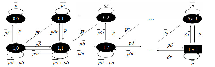
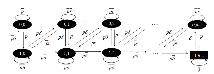
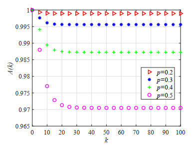
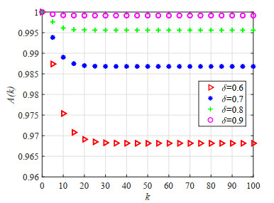
As an effective means to improve system reliability, cold standby redundancy design has been applied in many fields. Studies on the reliability of systems with retrial mechanisms mainly focus on the assumption of continuous time, but for some engineering systems whose states cannot be continuously monitored, it is of great theoretical and practical value to establish and analyze the reliability model of the discrete-time cold standby repairable retrial system. In this paper, the lifetime, repair time, and retrial time of each component were described by geometric distribution, and the reliability and optimal design models of a discrete-time cold standby retrial system were developed. Two different models were proposed based on two types of priority rules. According to the discrete-time Markov process theory, the transition probability matrix of the system states was given. The availability, reliability function, mean time to first failure (MTTFF) of the system, and other performance measures were obtained using the iterative algorithm of the difference equation, and the generative function method, algorithms for calculating stationary probability, and transient probability of the system were designed. The particle swarm optimization (PSO) algorithm was used to determine the optimal values of the repair rate and retrial rate corresponding to the minimum value of the cost-benefit ratio. Moreover, numerical analysis was performed to show the influence of each parameter on the system reliability and the cost-benefit ratio. The reliability measures of the systems with and without retrial mechanism were analytically compared.
Citation: Mengrao Ma, Linmin Hu, Yuyu Wang, Fang Luo. Discrete-time stochastic modeling and optimization for reliability systems with retrial and cold standbys[J]. AIMS Mathematics, 2024, 9(7): 19692-19717. doi: 10.3934/math.2024961
As an effective means to improve system reliability, cold standby redundancy design has been applied in many fields. Studies on the reliability of systems with retrial mechanisms mainly focus on the assumption of continuous time, but for some engineering systems whose states cannot be continuously monitored, it is of great theoretical and practical value to establish and analyze the reliability model of the discrete-time cold standby repairable retrial system. In this paper, the lifetime, repair time, and retrial time of each component were described by geometric distribution, and the reliability and optimal design models of a discrete-time cold standby retrial system were developed. Two different models were proposed based on two types of priority rules. According to the discrete-time Markov process theory, the transition probability matrix of the system states was given. The availability, reliability function, mean time to first failure (MTTFF) of the system, and other performance measures were obtained using the iterative algorithm of the difference equation, and the generative function method, algorithms for calculating stationary probability, and transient probability of the system were designed. The particle swarm optimization (PSO) algorithm was used to determine the optimal values of the repair rate and retrial rate corresponding to the minimum value of the cost-benefit ratio. Moreover, numerical analysis was performed to show the influence of each parameter on the system reliability and the cost-benefit ratio. The reliability measures of the systems with and without retrial mechanism were analytically compared.

| [1] |
A. S. Alfa, I. T. Castro, Discrete time analysis of a repairable machine, J. Appl. Probab., 39 (2002), 503–516. https://doi.org/10.1239/jap/1034082123 doi: 10.1239/jap/1034082123

|
| [2] |
J. R. Artalejo, A. Gómez-Corral, A note on the busy period of the M/G/1 queue with finite retrial group, Probab. Eng. Inform. Sc., 21 (2007), 77–82. https://doi.org/10.1017/S0269964807070052 doi: 10.1017/S0269964807070052
|
| [3] |
J. R. Artalejo, I. Atencia, P. Moreno, A discrete-time $\text{Geo}^\text{[X]}$/G/1 retrial queue with control of admission, Appl. Math. Model., 29 (2005), 1100–1120. https://doi.org/10.1016/j.apm.2005.02.005 doi: 10.1016/j.apm.2005.02.005
|
| [4] |
I. Atencia, P. Moreno, A discrete-time Geo/G/1 retrial queue with general retrial times, Queueing Syst., 48 (2004), 5–21. https://doi.org/10.1023/b:ques.0000039885.12490.02 doi: 10.1023/b:ques.0000039885.12490.02
|
| [5] |
I. Atencia, P. Moreno, A single-server G-queue in discrete-time with geometrical arrival and service process, Perform. Evaluation, 59 (2005), 85–97. https://doi.org/10.1016/j.peva.2004.07.019 doi: 10.1016/j.peva.2004.07.019
|
| [6] |
K. Avrachenkov, U. Yechiali, Retrial networks with finite buffers and their application to internet data traffic, Probab. Eng. Inform. Sc., 22 (2008), 519–536. https://doi.org/10.1017/S0269964808000314 doi: 10.1017/S0269964808000314
|
| [7] |
C. Bracquemond, O. Gaudoin, A survey on discrete lifetime distributions, Int. J. Reliab. Qual. Sa., 10 (2003), 69–98. https://doi.org/10.1142/S0218539303001007 doi: 10.1142/S0218539303001007
|
| [8] |
K. L. Bruning, Determining the discrete-time reliability of a repairable 2-out-of-(N+ 1): F system, IEEE T. Reliab., 45 (1996), 150–155. https://doi.org/10.1109/24.488934 doi: 10.1109/24.488934
|
| [9] |
W. L. Chen, K. H. Wang, Reliability analysis of a retrial machine repair problem with warm standbys and a single server with N-policy, Reliab. Eng. Syst. Safe., 180 (2018), 476–486. https://doi.org/10.1016/j.ress.2018.08.011 doi: 10.1016/j.ress.2018.08.011
|
| [10] |
G. I. Falin, A survey of retrial queues, Queueing Syst., 7 (1990), 127–167. https://doi.org/10.1007/BF01158472 doi: 10.1007/BF01158472
|
| [11] |
G. I. Falin, J. R. Artalejo, A finite source retrial queue, Eur. J. Oper. Res., 108 (1998), 409–424. https://doi.org/10.1016/S0377-2217(97)00170-7 doi: 10.1016/S0377-2217(97)00170-7
|
| [12] |
S. Gao, J. T. Wang, Reliability and availability analysis of a retrial system with mixed standbys and an unreliable repair facility, Reliab. Eng. Syst. Safe., 205 (2021), 107240. https://doi.org/10.1016/j.ress.2020.107240 doi: 10.1016/j.ress.2020.107240
|
| [13] |
S, Gao, J. T. Wang, T. V. Do, Analysis of a discrete-time repairable queue with disasters and working breakdowns, RAIRO-Oper. Res., 53 (2019), 1197–1216. https://doi.org/10.1051/ro/2018057 doi: 10.1051/ro/2018057
|
| [14] |
S. Gao, Availability and reliability analysis of a retrial system with warm standbys and second optional repair service, Commun. Stat-Theor. M., 52 (2021), 1039–1057. https://doi.org/10.1080/03610926.2021.1922702 doi: 10.1080/03610926.2021.1922702
|
| [15] |
A. Habib, R. Alsieidi, G. Youssef, Reliability analysis of a consecutive $r$-out-of-$n$: F system based on neural networks, Chaos Soliton. Fract., 39 (2009), 610–624. https://doi.org/10.1016/j.chaos.2007.01.151 doi: 10.1016/j.chaos.2007.01.151
|
| [16] |
C. Kan, S. Eryilmaz, Reliability assessment of a discrete time cold standby repairable system, Top, 29 (2021), 613–628. https://doi.org/10.1007/s11750-020-00586-7 doi: 10.1007/s11750-020-00586-7
|
| [17] |
J. Kang, L. M. Hu, R. Peng, Y. Li, R. L. Tian, Availability and cost-benefit evaluation for a repairable retrial system with warm standbys and priority, Statistical Theory and Related Fields, 7 (2022), 164–175. https://doi.org/10.1080/24754269.2022.2152591 doi: 10.1080/24754269.2022.2152591
|
| [18] |
P. Kumar, M. Jain, R. K. Meena, Transient analysis and reliability modeling of fault-tolerant system operating under admission control policy with double retrial features and working vacation, ISA T., 134 (2023), 183–199. https://doi.org/10.1016/j.isatra.2022.09.011 doi: 10.1016/j.isatra.2022.09.011
|
| [19] |
S. J. Lan, Y. H. Tang, An unreliable discrete-time retrial queue with probabilistic preemptive priority, balking customers and replacements of repair times, AIMS Math., 5 (2020), 4322–4344. https://doi.org/10.3934/math.2020276 doi: 10.3934/math.2020276
|
| [20] |
M. J. Li, L. M. Hu, R. Peng, Z. X. Bai, Reliability modeling for repairable circular consecutive-$k$-out-of-$n$: F systems with retrial feature, Reliab. Eng. Syst. Safe., 216 (2021), 107957. https://doi.org/10.1016/j.ress.2021.107957 doi: 10.1016/j.ress.2021.107957
|
| [21] |
Y. Li, L. R. Cui, C. Lin, Modeling and analysis for multi-state systems with discrete-time Markov regime-switching, Reliab. Eng. Syst. Safe., 166 (2017), 41–49. https://doi.org/10.1016/j.ress.2017.03.024 doi: 10.1016/j.ress.2017.03.024
|
| [22] |
Y. W. Liu, K. C. Kapur, Reliability measures for dynamic multistate nonrepairable systems and their applications to system performance evaluation, IIE Trans., 38 (2006), 511–520. https://doi.org/10.1080/07408170500341288 doi: 10.1080/07408170500341288
|
| [23] |
P. Moreno, A discrete-time retrial queue with unreliable server and general server lifetime, J. Math. Sci., 132 (2006), 643–655. https://doi.org/10.1007/s10958-006-0009-x doi: 10.1007/s10958-006-0009-x
|
| [24] |
T. Nakagawa, S. Osaki, The discrete Weibull distribution, IEEE T. Reliab., 24 (1975), 300–301. https://doi.org/10.1109/TR.1975.5214915 doi: 10.1109/TR.1975.5214915
|
| [25] |
W. J. Padgett, J. D. Spurrier, On discrete failure models, IEEE T. Reliab., 34 (1985), 253–256. https://doi.org/10.1109/TR.1985.5222137 doi: 10.1109/TR.1985.5222137
|
| [26] |
J. E. Ruiz-Castro, Complex multi-state systems modelled through marked Markovian arrival processes, Eur. J. Oper. Res., 252 (2016), 852–865. https://doi.org/10.1016/j.ejor.2016.02.007 doi: 10.1016/j.ejor.2016.02.007
|
| [27] |
J. E. Ruiz-Castro, G. Fernández-Villodre, A complex discrete warm standby system with loss of units, Eur. J. Oper. Res., 218 (2012), 456–469. https://doi.org/10.1016/j.ejor.2011.11.020 doi: 10.1016/j.ejor.2011.11.020
|
| [28] |
J. E. Ruiz-Castro, Q. L. Li, Algorithm for a general discrete $k$-out-of-$n$: G system subject to several types of failure with an indefinite number of repairpersons, Eur. J. Oper. Res., 211 (2011), 97–111. https://doi.org/10.1016/j.ejor.2010.10.024 doi: 10.1016/j.ejor.2010.10.024
|
| [29] |
J. E. Ruiz-Castro, G. Fernández-Villodre, R. Pérez-Ocón, A multi-component general discrete system subject to different types of failures with loss of units, Discrete Event Dyn. Syst., 19 (2009), 31–65. https://doi.org/10.1007/s10626-008-0046-3 doi: 10.1007/s10626-008-0046-3
|
| [30] |
J. E. Ruiz-Castro, G. Fernández-Villodre, R. Pérez-Ocón, Discrete repairable systems with external and internal failures under phase-type distributions, IEEE T. Reliab., 58 (2009), 41–52. https://doi.org/10.1109/TR.2008.2011667 doi: 10.1109/TR.2008.2011667
|
| [31] |
J. E. Ruiz-Castro, R. Pérez-Ocón, G. Fernández-Villodre, Modelling a reliability system governed by discrete phase-type distributions, Reliab. Eng. Syst. Safe., 93 (2008), 1650–1657. https://doi.org/10.1016/j.ress.2008.01.005 doi: 10.1016/j.ress.2008.01.005
|
| [32] |
A. A. Salvia, R. C. Bollinger, On discrete hazard functions, IEEE T. Reliab., 31 (1982), 458–459. https://doi.org/10.1109/TR.1982.5221432 doi: 10.1109/TR.1982.5221432
|
| [33] |
N. P. Sherman, J. P. Kharoufeh, M. A. Abramson, An M/G/1 retrial queue with unreliable server for streaming multimedia applications., Probab. Eng. Inform. Sc., 23 (2009), 281–304. https://doi.org/10.1017/S0269964809000175 doi: 10.1017/S0269964809000175
|
| [34] |
W. E. Stein, R. Dattero, A new discrete Weibull distribution, IEEE T. Reliab., 33 (1984), 196–197. https://doi.org/10.1109/TR.1984.5221777 doi: 10.1109/TR.1984.5221777
|
| [35] |
Y. H. Tang, M. M. Yu, X. Yun, S. J. Huang, Reliability indices of discrete-time $\text{Geo}^\text{[X]}$/G/1 queueing system with unreliable service station and multiple adaptive delayed vacations, J. Syst. Sci. Complex., 25 (2012), 1122–1135. https://doi.org/10.1007/s11424-012-1062-9 doi: 10.1007/s11424-012-1062-9
|
| [36] |
Y. H. Tang, X. Yun, S. J. Huang, Discrete-time $\text{Geo}^\text{[X]}$/G/1 queue with unreliable server and multiple adaptive delayed vacations, J. Comput. Appl. Math., 220 (2008), 439–455. https://doi.org/10.1016/j.cam.2007.08.019 doi: 10.1016/j.cam.2007.08.019
|
| [37] |
Y. Wang, L. M. Hu, L. Yang, J. Li, Reliability modeling and analysis for linear consecutive-$k$-out-of-$n$: F retrial systems with two maintenance activities, Reliab. Eng. Syst. Safe., 226 (2022), 108665. https://doi.org/10.1016/j.ress.2022.108665 doi: 10.1016/j.ress.2022.108665
|
| [38] |
Y. Wang, L. M. Hu, B. Zhao, R. L. Tian, Stochastic modeling and cost-benefit evaluation of consecutive $k$-out-of-$n$: F repairable retrial systems with two-phase repair and vacation, Comput. Ind. Eng., 175 (2023), 108851. https://doi.org/10.1016/j.cie.2022.108851 doi: 10.1016/j.cie.2022.108851
|
| [39] |
C. H. Wu, T. C. Yen, K. H. Wang, Availability and comparison of four retrial systems with imperfect coverage and general repair times, Reliab. Eng. Syst. Safe., 212 (2021), 107642. https://doi.org/10.1016/j.ress.2021.107642 doi: 10.1016/j.ress.2021.107642
|
| [40] |
J. B. Wu, J. X. Wang, Z. M. Liu, A discrete-time Geo/G/1 retrial queue with preferred and impatient customers, Appl. Math. Model., 37 (2013), 2552–2561. https://doi.org/10.1016/j.apm.2012.06.011 doi: 10.1016/j.apm.2012.06.011
|
| [41] |
E. Xekalaki, Hazard functions and life distributions in discrete time, Commun. Stat-Theor. M., 12 (1983), 2503–2509. https://doi.org/10.1080/03610928308828617 doi: 10.1080/03610928308828617
|
| [42] |
D. Y. Yang, C. L. Tsao, Reliability and availability analysis of standby systems with working vacations and retrial of failed components, Reliab. Eng. Syst. Safe., 182 (2019), 46–55. https://doi.org/10.1016/j.ress.2018.09.020 doi: 10.1016/j.ress.2018.09.020
|
| [43] |
T. C. Yen, K. H. Wang, C. H. Wu, Reliability-based measure of a retrial machine repair problem with working breakdowns under the F-policy, Comput. Ind. Eng., 150 (2020), 106885. https://doi.org/10.1016/j.cie.2020.106885 doi: 10.1016/j.cie.2020.106885
|
| [44] |
X. Y. Yu, L. M. Hu, M. R. Ma, Reliability measures of discrete time $k$-out-of-$n$: G retrial systems based on Bernoulli shocks, Reliab. Eng. Syst. Safe., 239 (2023), 109491. https://doi.org/10.1016/j.ress.2023.109491 doi: 10.1016/j.ress.2023.109491
|
Figures(23) / Tables(5)

Mengrao Ma, Linmin Hu, Yuyu Wang, Fang Luo. Discrete-time stochastic modeling and optimization for reliability systems with retrial and cold standbys[J]. AIMS Mathematics, 2024, 9(7): 19692-19717. doi: 10.3934/math.2024961


 DownLoad: