Dynamic analysis and optimal control of Zika virus transmission with immigration

Zongmin Yue; Yitong Li; Fauzi Mohamed Yusof; Zongmin Yue; Yitong Li; Fauzi Mohamed Yusof

doi:10.3934/math.20231116

AIMS Mathematics

2023, Volume 8, Issue 9: 21893-21913. doi: 10.3934/math.20231116

Previous Article Next Article

Research article Special Issues

Dynamic analysis and optimal control of Zika virus transmission with immigration

1.
Department of Mathematics, Shaanxi University of Science and Technology, Xi'an, 710021, China
2.
Faculty of Science and Mathematics, Sultan Idris Education University, Tanjong Malim, Malaysia

Received: 27 March 2023 Revised: 07 June 2023 Accepted: 28 June 2023 Published: 10 July 2023
MSC : 34D23, 34D20, 34D45, 92B05

In this paper, a type of Zika virus model with immigration is considered. Additionally based on the risk of infected immigrants, we propose a control measure of screening for immigrants and a three-measure control model of combined mosquito prevention and killing. The existence and stability of the equilibrium in the Zika virus model are analyzed. The necessary conditions for the existence of the optimal solution are given using Pontryagin's maximum principle. We focused on testing screening of the immigrating population to ensure a reduction in the transmission of the virus. Models have demonstrated that in combination with routine mosquito control measures and the appropriate use of mosquitoicides, the transmission of Zika virus in the population can be effectively reduced.
- Zika virus,
- immigration,
- stability,
- screening tests,
- optimal control
Citation: Zongmin Yue, Yitong Li, Fauzi Mohamed Yusof. Dynamic analysis and optimal control of Zika virus transmission with immigration[J]. AIMS Mathematics, 2023, 8(9): 21893-21913. doi: 10.3934/math.20231116

Related Papers:

Abstract

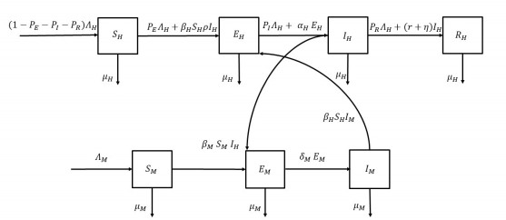
In this paper, a type of Zika virus model with immigration is considered. Additionally based on the risk of infected immigrants, we propose a control measure of screening for immigrants and a three-measure control model of combined mosquito prevention and killing. The existence and stability of the equilibrium in the Zika virus model are analyzed. The necessary conditions for the existence of the optimal solution are given using Pontryagin's maximum principle. We focused on testing screening of the immigrating population to ensure a reduction in the transmission of the virus. Models have demonstrated that in combination with routine mosquito control measures and the appropriate use of mosquitoicides, the transmission of Zika virus in the population can be effectively reduced.

References

[1]	G. W. Dick, S. F. Kitchen, A. J. Haddow, Zika virus (Ⅰ). Isolations and serological specificity, Trans. Roy. Soc. Trop. Med. H., 46 (1952), 509–520. https://doi.org/10.1016/0035-9203(52)90042-4 doi: 10.1016/0035-9203(52)90042-4
[2]	G. W. Dick, Zika virus (Ⅱ). Pathogenicity and physical properties, Trans. Roy. Soc. Trop. Med. H., 46 (1952), 521–534. http://dx.doi.org/10.1016/0035-9203(52)90043-6 doi: 10.1016/0035-9203(52)90043-6
[3]	D. Musso, C. Roche, E. Robin, T. Nhan, A. Teissier, V. M. Cao-Lormeau, Potential sexual transmission of Zika virus, Emerg. Infect. Dis., 21 (2015), 359–360. http://dx.doi.org/10.3201/eid2102.141363 doi: 10.3201/eid2102.141363
[4]	Y. S. Yan, Y. Q. Deng, Y. W. Weng, Zika virus infections in pregnant women are associated with microcephaly in newbowns, Chinese J. Zoonoses, 32 (2016), 107–108.
[5]	B. Rome, H. Laura, T. Butsaya, R. Wiriya, K. Chonticha, C. Piyawan, et al., Detection of Zika virus infection in Thailand, 2012–2014, Am. J. Trop. Med. Hyg., 93 (2015), 380–383. http://dx.doi.org/10.4269/ajtmh.15-0022 doi: 10.4269/ajtmh.15-0022
[6]	J. Tognarelli, S. Ulloa, E. Villagra, J. Lagos, C. Aguayo, R. Fasce, et al., A report on the outbreak of Zika virus on Easter Island, South Pacific, 2014, Arch. Virol., 161 (2016), 665–668. http://dx.doi.org/10.1007/s00705-015-2695-5 doi: 10.1007/s00705-015-2695-5
[7]	D. Diallo, A. A. Sall, C. T. Diagne, O. Faye, O. Faye, Y. Ba, et al., Zika virus emergence in mosquitoes in southeastern Senegal, 2011, PloS One, 9 (2014), e109442. http://dx.doi.org/10.1371/journal.pone.0109442 doi: 10.1371/journal.pone.0109442
[8]	F. Brauer, P. Driessche, Models for transmission of disease with immigration of infectives, Math. Biosci., 171 (2001), 143–154. http://dx.doi.org/10.1016/S0025-5564(01)00057-8 doi: 10.1016/S0025-5564(01)00057-8
[9]	M. Ayana, R. Koya. The Impact of infective immigrants on the spread and dynamics of Zika viruss, Am. J. Appl. Math., 5 (2017), 145–153. http://dx.doi.org/10.11648/j.ajam.20170506.11 doi: 10.11648/j.ajam.20170506.11
[10]	A. Traoré, Analysis of a vector-borne disease model with human and vectors immigration, J. Appl. Math. Comput., 64 (2020), 411–428. http://dx.doi.org/10.1007/s12190-020-01361-4 doi: 10.1007/s12190-020-01361-4
[11]	A. Kouidere, O. Balatif, M. Rachik, Analysis and optimal control of a mathematical modeling of the spread of African swine fever virus with a case study of South Korea and cost-effectiveness, Chaos Soliton. Fract., 146 (2021), 110867. http://dx.doi.org/10.1016/j.chaos.2021.110867 doi: 10.1016/j.chaos.2021.110867
[12]	A. Kouidere, O. Balatif, M. Rachik, Cost-effectiveness of a mathematical modeling with optimal control approach of spread of COVID-19 pandemic: A case study in Peru, Chaos Soliton. Fract., 10 (2023), 100090. http://dx.doi.org/10.1016/J.CSFX.2022.100090 doi: 10.1016/J.CSFX.2022.100090
[13]	A. M. Abdulfatai, A. Fügenschuh, Optimal control of intervention strategies and cost effectiveness analysis for a Zika virus model, Oper. Res. Health Care, 18 (2018), 99–111. http://dx.doi.org/10.1016/j.orhc.2017.08.004 doi: 10.1016/j.orhc.2017.08.004
[14]	T. Y. Miyaoka, S. Lenhart, J. F. C. A. Meyer, Optimal control of vaccination in a vector-borne reaction-diffusion model applied to Zika virus, J. Math. Biol., 79 (2019), 1077–1104. http://dx.doi.org/10.1007/s00285-019-01390-z doi: 10.1007/s00285-019-01390-z
[15]	E. Bonyah, M. A. Khan. K. O. Okosun, S. Islam, A theoretical model for Zika virus transmission, PloS One, 12 (2017), 1–18. http://dx.doi.org/10.1371/journal.pone.0185540 doi: 10.1371/journal.pone.0185540
[16]	E. O. Alzahrani, W. Ahmad, M. A. Khan, S. J. Malebary, Optimal control strategies of Zika virus model with mutant, Commun. Nonlinear Sci., 93 (2021), 105532. http://dx.doi.org/10.1016/j.cnsns.2020.105532 doi: 10.1016/j.cnsns.2020.105532
[17]	X. C. Duan, H. Jung, X. Z. Li, M. Martcheva, Dynamics and optimal control of an age-structured SIRVS epidemic model, Math. Method. Appl. Sci., 43 (2020), 1–18. http://dx.doi.org/10.1002/mma.6190 doi: 10.1002/mma.6190
[18]	M. A. Khan, S. W. Shah, S. Ulah, J. F. Gómez-Aguilar, A dynamical model of asymptomatic carrier zika virus with optimal control strategies, Nonlinear Anal.-Real, 50 (2019), 144–170. http://dx.doi.org/10.1016/j.nonrwa.2019.04.006 doi: 10.1016/j.nonrwa.2019.04.006
[19]	Z. M. Yue, F. M. Yusof, S. Shafie, Transmission dynamics of Zika virus incorporating harvesting, Math. Biosci. Eng., 17 (2020), 6181–6202. http://dx.doi.org/ 10.3934/mbe.2020327 doi: 10.3934/mbe.2020327
[20]	J. Lasalle, The stability of dynamical systems, Society for Industrial and Appiled Mathematics, Philadelphia, 1976. http://dx.doi.org/10.1137/1021079
[21]	J. Karrakchou, M. Rachik, S. Gourari, Optimal control and infectiology: Application to an hiv/aids model, Appl. Math. Comput., 177 (2006), 807–818. http://dx.doi.org/10.1016/j.amc.2005.11.092 doi: 10.1016/j.amc.2005.11.092
[22]	K. S. Lee, K. S. Lashari, Stability analysis and optimal control of pine wilt disease with horizontal transmission in vector population, Appl. Math. Comput., 226 (2014), 793–804. http://dx.doi.org/10.1016/j.amc.2013.09.061 doi: 10.1016/j.amc.2013.09.061
[23]	L. S. Pontryagin, V. G. Boltyanskii, R. V. Gamkrelidze, E. F. Mishchenko, The mathematical theory of optimal processes, Wiley, New York, 1962.
[24]	W. H. Fleming, R. W. Rishel, Deterministic and stochastic optimal control, Bull. Am. Math. Soc., 82 (1976), 997–998.
[25]	N. M. Ferguson, Z. M. Cucunubá, I. Dorigatti, G. L. Nedjati-Gilani, C. A. Donnelly, M. G. Basáñez, et al., Countering the Zika epidemic in Latin America, Science, 353 (2016), 6297. http://dx.doi.org/10.1126/science.aag0219 doi: 10.1126/science.aag0219
[26]	Y. Li, L. Wang, L. Pang, S. Liu, The data fitting and optimal control of a hand, foot and mouth disease (HFMD) model with stage structure, Appl. Math. Comput., 276 (2016), 61–74. http://dx.doi.org/10.1016/j.amc.2015.11.090 doi: 10.1016/j.amc.2015.11.090
[27]	WHO, Global vector control response 2017–2030. Available from: https://www.who.int/publications/i/item/9789241512978.

Reader Comments

Your name:*

Email:*
© 2023 the Author(s), licensee AIMS Press. This is an open access article distributed under the terms of the Creative Commons Attribution License (http://creativecommons.org/licenses/by/4.0)