Single-index logistic model for high-dimensional group testing data

Changfu Yang; Wenxin Zhou; Wenjun Xiong; Junjian Zhang; Juan Ding; Changfu Yang; Wenxin Zhou; Wenjun Xiong; Junjian Zhang; Juan Ding

doi:10.3934/math.2025163

AIMS Mathematics

2025, Volume 10, Issue 2: 3523-3560. doi: 10.3934/math.2025163

Previous Article Next Article

Research article Special Issues

Single-index logistic model for high-dimensional group testing data

1.
School of Mathematics and Statistics, Guangxi Normal University, Guilin 541004, China
2.
School of Mathematics, Hohai University, Nanjing 210098, China
† Changfu Yang and Wenxin Zhou contributed equally to this work.

Received: 06 November 2024 Revised: 05 February 2025 Accepted: 11 February 2025 Published: 24 February 2025
MSC : 62G08, 62P10

Group testing is an efficient screening method that reduces the number of tests by pooling multiple samples, making it especially effective in low-prevalence settings. This strategy gained significant attention during the COVID-19 pandemic, and has since been applied to detect various infectious diseases, including HIV, chlamydia, gonorrhea, influenza, and Zika virus. In this paper, we introduce a semi-parametric logistic single-index model for analyzing high-dimensional group testing data, which is particularly flexible in capturing complex nonlinear relationships. The proposed method achieves variable selection by parameter regularization, which proves especially beneficial for extracting relevant information from high-dimensional data. The performance of the model is evaluated through simulations across four group testing strategies: master pool testing, Dorfman testing, halving testing, and array testing. Further validation is provided using real-world data. The results demonstrate that our approach offers a flexible and robust tool for analyzing high-dimensional group testing data, with important applications in epidemiology and public health.
- group testing,
- latent variable,
- single-index model,
- high-dimensional data,
- variable selection,
- EM algorithm
Citation: Changfu Yang, Wenxin Zhou, Wenjun Xiong, Junjian Zhang, Juan Ding. Single-index logistic model for high-dimensional group testing data[J]. AIMS Mathematics, 2025, 10(2): 3523-3560. doi: 10.3934/math.2025163

Related Papers:

Abstract

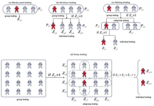
Group testing is an efficient screening method that reduces the number of tests by pooling multiple samples, making it especially effective in low-prevalence settings. This strategy gained significant attention during the COVID-19 pandemic, and has since been applied to detect various infectious diseases, including HIV, chlamydia, gonorrhea, influenza, and Zika virus. In this paper, we introduce a semi-parametric logistic single-index model for analyzing high-dimensional group testing data, which is particularly flexible in capturing complex nonlinear relationships. The proposed method achieves variable selection by parameter regularization, which proves especially beneficial for extracting relevant information from high-dimensional data. The performance of the model is evaluated through simulations across four group testing strategies: master pool testing, Dorfman testing, halving testing, and array testing. Further validation is provided using real-world data. The results demonstrate that our approach offers a flexible and robust tool for analyzing high-dimensional group testing data, with important applications in epidemiology and public health.

References

[1]	R. Dorfman, The detection of defective members of large populations, Ann. Math. Statist., 14 (1943), 436–440. http://dx.doi.org/10.1214/aoms/1177731363 doi: 10.1214/aoms/1177731363
[2]	S. Mallapaty, The mathematical strategy that could transform coronavirus testing, Nature, 583 (2020), 504–505. http://dx.doi.org/10.1038/d41586-020-02053-6 doi: 10.1038/d41586-020-02053-6
[3]	L. Mutesa, P. Ndishimye, Y. Butera, J. Souopgui, A. Uwineza, R. Rutayisire, et al., A pooled testing strategy for identifying SARS-CoV-2 at low prevalence, Nature, 589 (2021), 276–280. http://dx.doi.org/10.1038/s41586-020-2885-5 doi: 10.1038/s41586-020-2885-5
[4]	W. Chen, C. Tatsuoka, X. Lu, HiBGT: High-performance Bayesian group testing for COVID-19, In: 2022 IEEE 29th international conference on high performance computing, data, and analytics (HiPC), 2022,176–185. https://doi.org/10.1109/HiPC56025.2022.00033
[5]	D. J. Westreich, M. G. Hudgens, S. A. Fiscus, C. D. Pilcher, Optimizing screening for acute human immunodeficiency virus infection with pooled nucleic acid amplification tests, J. Clin. Microbiol., 46 (2008), 1785–1792. http://dx.doi.org/10.1128/jcm.00787-07 doi: 10.1128/jcm.00787-07
[6]	M. Krajden, D. Cook, A. Mak, K. Chu, N. Chahil, M. Steinberg, et al., Pooled nucleic acid testing increases the diagnostic yield of acute HIV infections in a high-risk population compared to 3rd and 4th generation HIV enzyme immunoassays, J. Clin. Virol., 61 (2014), 132–137. http://dx.doi.org/10.1016/j.jcv.2014.06.024 doi: 10.1016/j.jcv.2014.06.024
[7]	J. L. Lewis, V. M. Lockary, S. Kobic, Cost savings and increased efficiency using a stratified specimen pooling strategy for Chlamydia trachomatis and Neisseria gonorrhoeae, Sex. Transm. Dis., 39 (2012), 46–48. http://dx.doi.org/10.1097/OLQ.0b013e318231cd4a doi: 10.1097/OLQ.0b013e318231cd4a
[8]	T. T. Van, J. Miller, D. M. Warshauer, E. Reisdorf, D. Jernigan, R. Humes, et al., Pooling Nasopharyngeal/Throat swab specimens to increase testing capacity for influenza viruses by PCR, J. Clin. Microbiol., 50 (2012), 891–896. http://dx.doi.org/10.1128/jcm.05631-11 doi: 10.1128/jcm.05631-11
[9]	P. Saá, M. Proctor, G. Foster, D. Krysztof, C. Winton, J. M. Linnen, et al., Investigational testing for Zika virus among U.S. blood donors, N. Engl. J. Med., 378 (2018), 1778–1788. http://dx.doi.org/10.1056/NEJMoa1714977 doi: 10.1056/NEJMoa1714977
[10]	J. M. Tebbs, C. S. McMahan, C. R. Bilder, Two-stage hierarchical group testing for multiple infections with application to the infertility prevention project, Biometrics, 69 (2013), 1064–1073. http://dx.doi.org/10.1111/biom.12080 doi: 10.1111/biom.12080
[11]	C. S. McMahan, J. M. Tebbs, T. E. Hanson, C. R. Bilder, Bayesian regression for group testing data, Biometrics, 73 (2017), 1443–1452. http://dx.doi.org/10.1111/biom.12704 doi: 10.1111/biom.12704
[12]	A. Yuan, J. Piao, J. Ning, J. Qin, Semiparametric isotonic regression modelling and estimation for group testing data, Can. J. Stat., 49 (2021), 659–677. http://dx.doi.org/10.1002/cjs.11581 doi: 10.1002/cjs.11581
[13]	J. Ding, W. J. Xiong, Robust group testing for multiple traits with misclassification, J. Appl. Stat., 42 (2015), 2115–2125. https://doi.org/10.1080/02664763.2015.1019841 doi: 10.1080/02664763.2015.1019841
[14]	S. C. Mokalled, C. S. McMahan, J. M. Tebbs, D. Andrew Brown, C. R. Bilder, Incorporating the dilution effect in group testing regression, Stat. Med., 40 (2021), 2540–2555. http://dx.doi.org/10.1002/sim.8916 doi: 10.1002/sim.8916
[15]	X. Z. Huang, M. S. S. Warasi, Maximum likelihood estimators in regression models for error-prone group testing data, Scand. J. Stat., 44 (2017), 918–931. http://dx.doi.org/10.1111/sjos.12282 doi: 10.1111/sjos.12282
[16]	G. Haber, Y. Malinovsky, P. S. Albert, Sequential estimation in the group testing problem, Sequential Anal., 37 (2018), 1–17. http://dx.doi.org/10.1080/07474946.2017.1394716 doi: 10.1080/07474946.2017.1394716
[17]	J. L. Horowitz, Semiparametric and nonparametric methods in econometrics, 1 Eds., New York: Springer, 2009. https://doi.org/10.1007/978-0-387-92870-8
[18]	P. Radchenko, High dimensional single index models, J. Multivariate Anal., 139 (2015), 266–282. http://dx.doi.org/10.1016/j.jmva.2015.02.007 doi: 10.1016/j.jmva.2015.02.007
[19]	Z. C. Elmezouar, F. Alshahrani, I. M. Almanjahie, S. Bouzebda, Z. Kaid, A. Laksaci, Strong consistency rate in functional single index expectile model for spatial data, AIMS Mathematics, 9 (2024), 5550–5581. http://dx.doi.org/10.3934/math.2024269 doi: 10.3934/math.2024269
[20]	Y. N. Chen, R. J. Samworth, Generalized additive and index models with shape constraints, J. R. Stat. Soc. Ser. B Stat. Methodol., 78 (2016), 729–754. http://dx.doi.org/10.1111/rssb.12137 doi: 10.1111/rssb.12137
[21]	Z. Kereta, T. Klock, V. Naumova, Nonlinear generalization of the monotone single index model, Inf. Inference, 10 (2021), 987–1029. http://dx.doi.org/10.1093/imaiai/iaaa013 doi: 10.1093/imaiai/iaaa013
[22]	D. Wang, C. S. McMahan, C. M. Gallagher, A general regression framework for group testing data, which incorporates pool dilution effects, Stat. Med., 34 (2015), 3606–3621. http://dx.doi.org/10.1002/sim.6578 doi: 10.1002/sim.6578
[23]	K. B. Gregory, D. Wang, C. S. McMahan, Adaptive elastic net for group testing, Biometrics, 75 (2019), 13–23. http://dx.doi.org/10.1111/biom.12973 doi: 10.1111/biom.12973
[24]	H. Ko, K. Kim, H. Sun, Multiple group testing procedures for analysis of high-dimensional genomic data, Genomics Inform., 14 (2016), 187–195. http://dx.doi.org/10.5808/gi.2016.14.4.187 doi: 10.5808/gi.2016.14.4.187
[25]	A. Delaigle, P. Hall, Nonparametric methods for group testing data, taking dilution into account, Biometrika, 102 (2015), 871–887. http://dx.doi.org/10.1093/biomet/asv049 doi: 10.1093/biomet/asv049
[26]	S. Self, C. McMahan, S. Mokalled, Capturing the pool dilution effect in group testing regression: A Bayesian approach, Stat. Med., 41 (2022), 4682–4696. http://dx.doi.org/10.1002/sim.9532 doi: 10.1002/sim.9532
[27]	X. L. Zuo, J. Ding, J. J. Zhang, W. J. Xiong, Nonparametric additive regression for high-dimensional group testing data, Mathematics, 12 (2024), 686. http://dx.doi.org/10.3390/math12050686 doi: 10.3390/math12050686
[28]	R. J. Carroll, J. Fan, I. Gijbels, M. P. Wand, Generalized partially linear single-index models, J. Amer. Statist. Assoc., 92 (1997), 477–489. https://doi.org/10.1080/01621459.1997.10474001 doi: 10.1080/01621459.1997.10474001
[29]	L. Zhu, L. Xue, Empirical likelihood confidence regions in a partially linear single-index model, J. R. Stat. Soc. Ser. B Stat. Methodol., 68 (2006), 549–570. https://doi.org/10.1111/j.1467-9868.2006.00556.x doi: 10.1111/j.1467-9868.2006.00556.x
[30]	W. Lin, K. B. Kulasekera, Identifiability of single-index models and additive-index models, Biometrika, 94 (2007), 496–501. https://doi.org/10.1093/biomet/asm029 doi: 10.1093/biomet/asm029
[31]	X. Cui, W. K. Härdle, L. X. Zhu, The EFM approach for single-index models, Ann. Statist., 39 (2011), 1658–1688. http://dx.doi.org/10.1214/10-aos871 doi: 10.1214/10-aos871
[32]	X. Guo, C. Z. Niu, Y. P. Yang, W. L. Xu, Empirical likelihood for single index model with missing covariates at random, Statistics, 49 (2015), 588–601. http://dx.doi.org/10.1080/02331888.2014.881826 doi: 10.1080/02331888.2014.881826
[33]	W. Xiong, J. Ding, W. Zhang, A. Liu, Q. Li, Nested group testing procedure, Commun. Math. Stat., 11 (2023), 663–693. http://dx.doi.org/10.1007/s40304-021-00269-0 doi: 10.1007/s40304-021-00269-0
[34]	J. X. Lin, D. W. Wang, Q. Zheng, Regression analysis and variable selection for two-stage multiple-infection group testing data, Stat. Med., 38 (2019), 4519–4533. http://dx.doi.org/10.1002/sim.8311 doi: 10.1002/sim.8311
[35]	D. Wang, C. S. McMahan, C. M. Gallagher, K. B. Kulasekera, Semiparametric group testing regression models, Biometrika, 101 (2014), 587–598. https://doi.org/10.1093/biomet/asu007 doi: 10.1093/biomet/asu007
[36]	B. A. Zhang, C. R. Bilder, J. M. Tebbs, Group testing regression model estimation when case identification is a goal, Biometrical J., 55 (2013), 173–189. http://dx.doi.org/10.1002/bimj.201200168 doi: 10.1002/bimj.201200168
[37]	S. Vansteelandt, E. Goetghebeur, T. Verstraeten, Regression models for disease prevalence with diagnostic tests on pools of serum samples, Biometrics, 56 (2000), 1126–1133. http://dx.doi.org/10.1111/j.0006-341x.2000.01126.x doi: 10.1111/j.0006-341x.2000.01126.x
[38]	C. Boor, A practical guide to splines, New York: Springer, 1978.
[39]	R. Tibshirani, Regression shrinkage and selection via the Lasso, J. R. Stat. Soc. Ser. B Stat. Methodol., 58 (1996), 267–288. http://dx.doi.org/10.1111/j.2517-6161.1996.tb02080.x doi: 10.1111/j.2517-6161.1996.tb02080.x
[40]	J. Fan, R. Z. Li, Variable selection via nonconcave penalized likelihood and its Oracle properties, J. Amer. Statist. Assoc., 96 (2001), 1348–1360. http://dx.doi.org/10.1198/016214501753382273 doi: 10.1198/016214501753382273
[41]	C. H. Zhang, Nearly unbiased variable selection under minimax concave penalty, Ann. Statist., 38 (2010), 894–942. http://dx.doi.org/10.1214/09-aos729 doi: 10.1214/09-aos729
[42]	W. C. Guo, X. H. Zhou, S. J. Ma, Estimation of optimal individualized treatment rules using a covariate-specific treatment effect curve with high-dimensional covariates, J. Amer. Statist. Assoc., 116 (2021), 309–321. http://dx.doi.org/10.1080/01621459.2020.1865167 doi: 10.1080/01621459.2020.1865167
[43]	J. Duchi, E. Hazan, Y. Singer, Adaptive subgradient methods for online learning and stochastic optimization, J. Mach. Learn. Res., 12 (2011), 2121–2159.
[44]	P. Breheny, J. Huang, Coordinate descent algorithms for nonconvex penalized regression, with applications to biological feature selection, Ann. Appl. Stat., 5 (2011), 232–253. http://dx.doi.org/10.1214/10-aoas388 doi: 10.1214/10-aoas388
[45]	S. J. Guan, M. T. Zhao, Y. H. Cui, Variable selection for single-index varying-coefficients models with applications to synergistic G x E interactions, Electron. J. Statist., 17 (2023), 823–857. http://dx.doi.org/10.1214/23-ejs2117 doi: 10.1214/23-ejs2117
[46]	L. Wang, L. J. Yang, Spline estimation of single-index models, Statist. Sinica, 19 (2009), 765–783.
[47]	K. N. Turi, D. M. Buchner, D. S. Grigsby-Toussaint, Predicting risk of type 2 diabetes by using data on easy-to-measure risk factors, Prev. Chronic. Dis., 14 (2017), 160244. http://dx.doi.org/10.5888/pcd14.160244 doi: 10.5888/pcd14.160244
[48]	K. Bai, X. Chen, R. Song, W. Shi, S. Shi, Association of body mass index and waist circumference with type 2 diabetes mellitus in older adults: a cross-sectional study, BMC Geriatr., 22 (2022), 489. http://dx.doi.org/10.1186/s12877-022-03145-w doi: 10.1186/s12877-022-03145-w
[49]	M. B. Snijder, P. Z. Zimmet, M. Visser, J. M. Dekker, J. C. Seidell, J. E. Shaw, Independent and opposite associations of waist and hip circumferences with diabetes, hypertension and dyslipidemia: the AusDiab Study, Int. J. Obes., 28 (2004), 402–409. http://dx.doi.org/10.1038/sj.ijo.0802567 doi: 10.1038/sj.ijo.0802567
[50]	C. Wittenbecher, O. Kuxhaus, H. Boeing, N. Stefan, M. B. Schulze, Associations of short stature and components of height with incidence of type 2 diabetes: Mediating effects of cardiometabolic risk factors, Diabetologia, 62 (2019), 2211–2221. https://doi.org/10.1007/s00125-019-04978-8 doi: 10.1007/s00125-019-04978-8
[51]	G. Colussi, A. Da Porto, A. Cavarape, Hypertension and type 2 diabetes: Lights and shadows about causality, J. Hum. Hypertens., 34 (2020), 91–93. http://dx.doi.org/10.1038/s41371-019-0268-x doi: 10.1038/s41371-019-0268-x
[52]	S. E. Richards, C. Wijeweera, A. Wijeweera, Lifestyle and socioeconomic determinants of diabetes: Evidence from country-level data, PLoS ONE, 17 (2022), e0270476. https://doi.org/10.1371/journal.pone.0270476 doi: 10.1371/journal.pone.0270476
[53]	J. Su, J. Y. Zhou, R. Tao, Y. N. Wan, Y. Qin, Y. Lu, et al., Association between family history of diabetes and incident diabetes of adults: A prospective study, Chin. J. Prev. Med., 54 (2020), 828–833. https://doi.org/10.3760/cma.j.cn112150-20200212-00091 doi: 10.3760/cma.j.cn112150-20200212-00091
[54]	S. Clotet-Freixas, O. Zaslaver, M. Kotlyar, C. Pastrello, A. T Quaile, C. M. McEvoy, et al., Sex differences in kidney metabolism may reflect sex-dependent outcomes in human diabetic kidney disease, Sci. Transl. Med., 16 (2024), eabm2090. https://doi.org/10.1126/scitranslmed.abm2090 doi: 10.1126/scitranslmed.abm2090
[55]	M. Yu, T. Liu, R. Valdez, M. Gwinn, M. J. Khoury, Application of support vector machine modeling for prediction of common diseases: The case of diabetes and pre-diabetes, BMC Med. Inform. Decis. Mak., 10 (2010), 16. https://doi.org/10.1186/1472-6947-10-16 doi: 10.1186/1472-6947-10-16
[56]	K. K. Aldossari, A. Aldiab, J. M. Al-Zahrani, S. H. Al-Ghamdi, M. Abdelrazik, M. A. Batais, et al., Prevalence of prediabetes, diabetes, and its associated risk factors among males in Saudi Arabia: A population-based survey, J. Diabetes Res., 2018 (2018), 2194604. https://doi.org/10.1155/2018/2194604 doi: 10.1155/2018/2194604
[57]	F. S. Yen, J. C. C. Wei, J. S. Liu, C. M. Hwu, Parental income level and risk of developing type 2 diabetes in youth, JAMA Netw. Open., 6 (2023), e2345812. https://doi.org/10.1001/jamanetworkopen.2023.45812 doi: 10.1001/jamanetworkopen.2023.45812

Reader Comments

Your name:*

Email:*
© 2025 the Author(s), licensee AIMS Press. This is an open access article distributed under the terms of the Creative Commons Attribution License (http://creativecommons.org/licenses/by/4.0)