3D-Chaotic discrete system of vector borne diseases using environment factor with deep analysis

Shaymaa H. Salih; Nadia M. G. Al-Saidi; Shaymaa H. Salih; Nadia M. G. Al-Saidi

doi:10.3934/math.2022219

AIMS Mathematics

2022, Volume 7, Issue 3: 3972-3987. doi: 10.3934/math.2022219

Previous Article Next Article

Research article Special Issues

3D-Chaotic discrete system of vector borne diseases using environment factor with deep analysis

Shaymaa H. Salih ¹,
Nadia M. G. Al-Saidi ^{2
,
,}

1.
Department of Mathematics, College of Science, Mustansiriyah University, Iraq
2.
Department of Applied Sciences, University of Technology, Iraq

Received: 08 October 2021 Accepted: 17 November 2021 Published: 13 December 2021
MSC : 37M20, 34H10

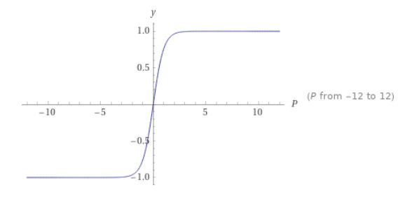
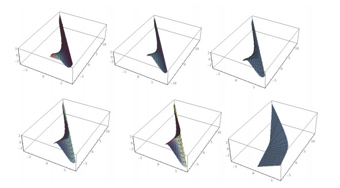
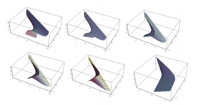
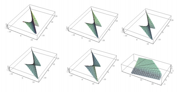
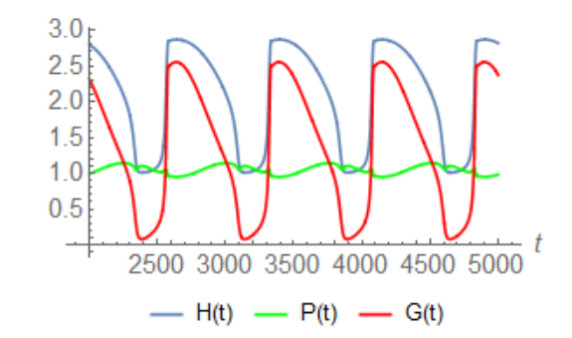
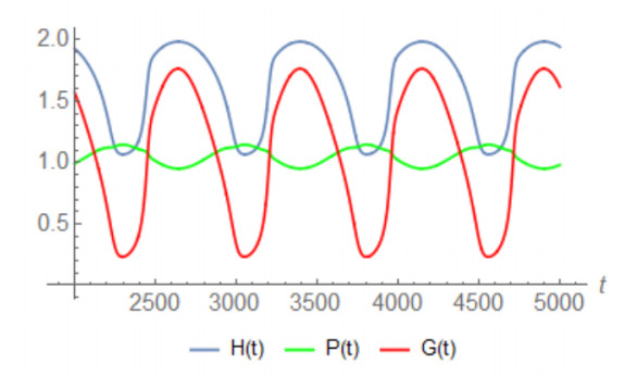
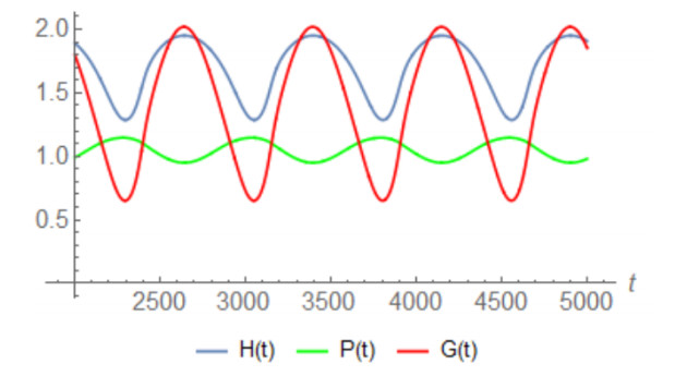
Vector-Borne Disease (VBD) is a disease that consequences as of an infection communicated to humans and other animals by blood-feeding anthropoids, like mosquitoes, fleas, and ticks. Instances of VBDs include Dengue infection, Lyme infection, West Nile virus, and malaria. In this effort, we formulate a parametric discrete-time chaotic system that involves an environmental factor causing VBD. Our suggestion is to study how the inclusion of the parasitic transmission media (PTM) in the system would impact the analysis results. We consider a chaotic formula of the PTM impact, separating two types of functions, the host and the parasite. The considered applications are typically characterized by chaotic dynamics, and thus chaotic systems are suitable for their modeling, with corresponding model parameters, that depend on control measures. Dynamical performances of the suggested system and its global stability are considered.
- differential operator,
- fractal chaotic system,
- fractal,
- locally fractional calculus,
- fractal dynamic system,
- difference system
Citation: Shaymaa H. Salih, Nadia M. G. Al-Saidi. 3D-Chaotic discrete system of vector borne diseases using environment factor with deep analysis[J]. AIMS Mathematics, 2022, 7(3): 3972-3987. doi: 10.3934/math.2022219

Related Papers:

Abstract

Vector-Borne Disease (VBD) is a disease that consequences as of an infection communicated to humans and other animals by blood-feeding anthropoids, like mosquitoes, fleas, and ticks. Instances of VBDs include Dengue infection, Lyme infection, West Nile virus, and malaria. In this effort, we formulate a parametric discrete-time chaotic system that involves an environmental factor causing VBD. Our suggestion is to study how the inclusion of the parasitic transmission media (PTM) in the system would impact the analysis results. We consider a chaotic formula of the PTM impact, separating two types of functions, the host and the parasite. The considered applications are typically characterized by chaotic dynamics, and thus chaotic systems are suitable for their modeling, with corresponding model parameters, that depend on control measures. Dynamical performances of the suggested system and its global stability are considered.

References

[1]	Mattingly, P. Frederick, The biology of mosquito-borne disease, The biology of mosquito-borne disease, 1969. doi: 10.1136/bmj.1.5647.835.
[2]	C. Dye, Models for the population dynamics of the yellow fever mosquito, Aedes aegypti, J. Anim. Ecol., 53 (1984), 247-268. doi: 10.2307/4355. doi: 10.2307/4355
[3]	R. M. May, Biological populations with non overlapping generations: stable points, stable cycles, and chaos, Science, 186 (1974), 645-647. doi: 10.1126/science.186.4164.645. doi: 10.1126/science.186.4164.645
[4]	T. S. Bellows, The descriptive properties of some models for density dependence, J. Anim. Ecol., 50 (1981), 139-156. doi: 10.2307/4037. doi: 10.2307/4037
[5]	X. Ma, Q. Din, M. Rafaqat, N. Javaid, Y. Feng, A density-dependent host-parasitoid model with stability, bifurcation and chaos control, Mathematics, 8 (2020), 536. doi: 10.3390/math8040536. doi: 10.3390/math8040536
[6]	H. A. Jalab, R. W. Ibrahim, New activation functions for complex-valued neural network, Int. J. Phys. Sci., 6 (2011), 1766-1772.
[7]	R. W. Ibrahim, Utility function for intelligent access web selection using the normalized fuzzy fractional entropy, Soft Comput., (2020), 1-8.
[8]	Q. Din, Global behavior of a host-parasitoid model under the constant refuge effect, Appl. Math. Model., 40 (2016), 2815-2826. doi: 10.1016/j.apm.2015.09.012. doi: 10.1016/j.apm.2015.09.012
[9]	S. M. Sajjad, Q. Din, M. Safeer, M. Asif Khan, K. Ahmad, A dynamically consistent nonstandard finite difference scheme for a predator-prey model, Adv. Differ. Equ-NY, 1 (2019), 1-17. doi: 10.1186/s13662-019-2319-6. doi: 10.1186/s13662-019-2319-6
[10]	Q. Din, K. Haider, Discretization, bifurcation analysis and chaos control for Schnakenberg model, J. Math. Chem., 58 (2020), 1615-1649. doi: 10.1007/s10910-020-01154-x. doi: 10.1007/s10910-020-01154-x
[11]	M. Islam, Mathematical Modeling of the Garbage Collection Problem, Math. Model. Appl. Comput., 4 (2013), 29-38.
[12]	H. Natiq, N. M. G. Al-Saidi, M. R. M. Said, A. Kilicman, A new hyperchaotic map and its application for image encryption, Eur. phys. J. Plus, 133 (2018), 1-14. doi: 10.1140/epjp/i2018-11834-2. doi: 10.1140/epjp/i2018-11834-2
[13]	N. M. G. Al-Saidi, D. Younus, H. Natiq, M. R. K. Ariffin, Z. Mahad, A New hyperchaotic map for a secure communication scheme with an experimental realization, Symmetry, 12 (2020), 1881. doi: 10.3390/sym12111881. doi: 10.3390/sym12111881
[14]	A. K. Farhan, N. M. G. Al-Saidi, A. T. Maolood, F. Nazarimehr, I. Hussain, Entropy analysis and image encryption application based on a new chaotic system crossing a cylinder, Entropy, 21 (2019), 958. doi: 10.3390/e21100958. doi: 10.3390/e21100958
[15]	M. S. Fadhil, A. K. Farhan, M. N. Fadhil, N. M. G. Al-Saidi, A New Lightweight AES Using a Combination of Chaotic Systems, 2020 IEEE first conference on information Technology to Enhance E-learning and Other Applications (IT-ELA), (2020), 82-88.
[16]	P. S. Sadeghi, Z. Rostami, V. Pham, F. E. Alsaadi, T. Hayat, Modeling of neurodegenerative diseases using discrete chaotic systems, Commun. Theor. Phys., 71 (2019), 1241. doi: 10.1088/0253-6102/71/10/1241. doi: 10.1088/0253-6102/71/10/1241
[17]	R. W. Ibrahim, D. Altulea, Controlled homeodynamic concept using a conformable calculus in artificial biological systems, Chaos, Solitons Fract., 140 (2020), 110-132. doi: 10.1016/j.chaos.2020.110132. doi: 10.1016/j.chaos.2020.110132
[18]	L. Stephen, Dynamical Systems with Applications Using Mathematica, Boston: Birkhauser, 2007.
[19]	M. Mesbahi, G. P. Papavassilopoulos. On the rank minimization problem over a positive semidefinite linear matrix inequality, IEEE T. Automat. Contr., 42 (1997), 239-243. doi: 10.1109/9.554402. doi: 10.1109/9.554402
[20]	Z. Luo, J. Tao, N. Xiu, Lowest-rank solutions of continuous and discrete Lyapunov equations over symmetric cone, Linear Algebra Appl., 452 (2014), 68-88. doi: 10.1016/j.laa.2014.03.028. doi: 10.1016/j.laa.2014.03.028

Reader Comments

Your name:*

Email:*
© 2022 the Author(s), licensee AIMS Press. This is an open access article distributed under the terms of the Creative Commons Attribution License (http://creativecommons.org/licenses/by/4.0)