The widespread application of chaotic dynamical systems in different fields of science and engineering has attracted the attention of many researchers. Hence, understanding and capturing the complexities and the dynamical behavior of these chaotic systems is essential. The newly proposed fractal-fractional derivative and integral operators have been used in literature to predict the chaotic behavior of some of the attractors. It is argued that putting together the concept of fractional and fractal derivatives can help us understand the existing complexities better since fractional derivatives capture a limited number of problems and on the other side fractal derivatives also capture different kinds of complexities. In this study, we use the newly proposed Caputo-Fabrizio fractal-fractional derivatives and integral operators to capture and predict the behavior of the Lorenz chaotic system for different values of the fractional dimension $ q $ and the fractal dimension $ k $. We will look at the well-posedness of the solution. For the effect of the Caputo-Fabrizio fractal-fractional derivatives operator on the behavior, we present the numerical scheme to study the graphical numerical solution for different values of $ q $ and $ k $.
Citation: Anastacia Dlamini, Emile F. Doungmo Goufo, Melusi Khumalo. On the Caputo-Fabrizio fractal fractional representation for the Lorenz chaotic system[J]. AIMS Mathematics, 2021, 6(11): 12395-12421. doi: 10.3934/math.2021717
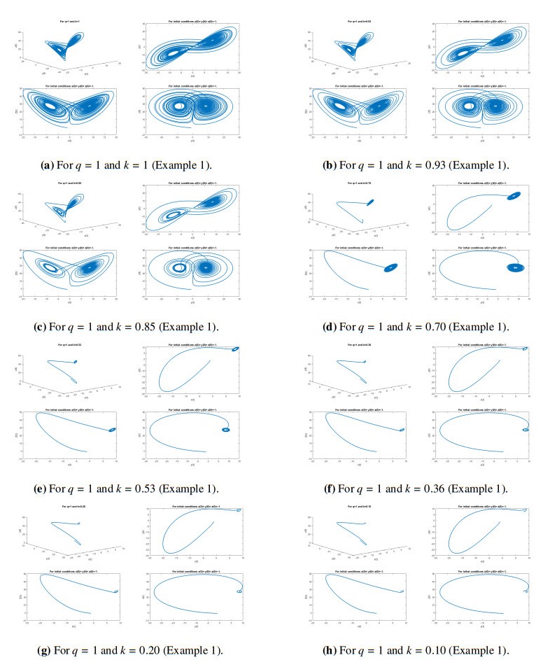
The widespread application of chaotic dynamical systems in different fields of science and engineering has attracted the attention of many researchers. Hence, understanding and capturing the complexities and the dynamical behavior of these chaotic systems is essential. The newly proposed fractal-fractional derivative and integral operators have been used in literature to predict the chaotic behavior of some of the attractors. It is argued that putting together the concept of fractional and fractal derivatives can help us understand the existing complexities better since fractional derivatives capture a limited number of problems and on the other side fractal derivatives also capture different kinds of complexities. In this study, we use the newly proposed Caputo-Fabrizio fractal-fractional derivatives and integral operators to capture and predict the behavior of the Lorenz chaotic system for different values of the fractional dimension $ q $ and the fractal dimension $ k $. We will look at the well-posedness of the solution. For the effect of the Caputo-Fabrizio fractal-fractional derivatives operator on the behavior, we present the numerical scheme to study the graphical numerical solution for different values of $ q $ and $ k $.

| [1] | R. E. Gutierrez, J. M. Rosario, J. Tenreiro Machado, Fractional order calculus: basic concepts and engineering applications, Math. Probl. Eng., 2010 (2010), 375858. |
| [2] |
M. Inc, A. Yusuf, A. I. Aliyu, D. Baleanu, Investigation of the logarithmic-KdV equation involving Mittag-Leffler type kernel with Atangana–Baleanu derivative, Physica A, 506 (2018), 520–531. doi: 10.1016/j.physa.2018.04.092

|
| [3] |
R. Almeida, N. R. Bastos, M. T. T. Monteiro, Modeling some real phenomena by fractional differential equations, Math. Method. Appl. Sci., 39 (2016), 4846–4855. doi: 10.1002/mma.3818
|
| [4] |
R. Almeida, A. B. Malinowska, M. T. T. Monteiro, Fractional differential equations with a Caputo derivative with respect to a kernel function and their applications, Math. Method. Appl. Sci., 41 (2018), 336–352. doi: 10.1002/mma.4617
|
| [5] |
A. Yusuf, S. Qureshi, M. Inc, A. I. Aliyu, D. Baleanu, A. A. Shaikh, Two-strain epidemic model involving fractional derivative with Mittag-Leffler kernel, Chaos, 28 (2018), 123121. doi: 10.1063/1.5074084
|
| [6] | M. Awadalla, Y. Yameni, Modeling exponential growth and exponential decay real phenomena by $\psi$-Caputo fractional derivative, JAMCS, 28 (2018), 1–13. |
| [7] |
A. Jajarmi, S. Arshad, D. Baleanu, A new fractional modelling and control strategy for the outbreak of dengue fever, Physica A, 535 (2019), 122524. doi: 10.1016/j.physa.2019.122524
|
| [8] | M. Khader, K. M. Saad, Numerical treatment for studying the blood ethanol concentration systems with different forms of fractional derivatives, Int. J. Mod. Phys. C, 31 (2020), https://doi.org/10.1142/S0129183120500448. |
| [9] | S. Bushnaq, S. A. Khan, K. Shah, G. Zaman, Existence theory of HIV-1 infection model by using arbitrary order derivative of without singular kernel type, Journal of Mathematical Analysis, 9 (2018), 16–28. |
| [10] |
S. Rezapour, H. Mohammadi, A study on the AH1N1/09 influenza transmission model with the fractional Caputo–Fabrizio derivative, Adv. Differ. Equ., 2020 (2020), 1–15. doi: 10.1186/s13662-019-2438-0
|
| [11] |
S. B. Chen, S. Rashid, M. A. Noor, R. Ashraf, Y. M. Chu, A new approach on fractional calculus and probability density function, AIMS Mathematics, 5 (2020), 7041–7054. doi: 10.3934/math.2020451
|
| [12] | S. Das, I. Pan, Fractional order signal processing: introductory concepts and applications, Springer Science $ & $ Business Media, 2011. |
| [13] |
F. Meral, T. Royston, R. Magin, Fractional calculus in viscoelasticity: an experimental study, Commun. Nonlinear Sci., 15 (2010), 939–945. doi: 10.1016/j.cnsns.2009.05.004
|
| [14] |
K. M. Owolabi, A. Atangana, On the formulation of Adams-Bashforth scheme with Atangana-Baleanu-Caputo fractional derivative to model chaotic problems, Chaos, 29 (2019), 023111. doi: 10.1063/1.5085490
|
| [15] |
M. Inc, A. Yusuf, A. I. Aliyu, D. Baleanu, Investigation of the logarithmic-KdV equation involving Mittag-Leffler type kernel with Atangana–Baleanu derivative, Physica A, 506 (2018), 520–531. doi: 10.1016/j.physa.2018.04.092
|
| [16] |
A. Atangana, A. Akgül, K. M. Owolabi, Analysis of fractal fractional differential equations, Alex. Eng. J., 59 (2020), 1117–1134. doi: 10.1016/j.aej.2020.01.005
|
| [17] |
A. Akgül, A novel method for a fractional derivative with non-local and non-singular kernel, Chaos Soliton. Fract., 114 (2018), 478–482. doi: 10.1016/j.chaos.2018.07.032
|
| [18] |
K. M. Owolabi, A. Atangana, Chaotic behaviour in system of noninteger-order ordinary differential equations, Chaos Soliton. Fract., 115 (2018), 362–370. doi: 10.1016/j.chaos.2018.07.034
|
| [19] |
K. M. Owolabi, Z. Hammouch, Spatiotemporal patterns in the Belousov–Zhabotinskii reaction systems with Atangana–Baleanu fractional order derivative, Physica A, 523 (2019), 1072–1090. doi: 10.1016/j.physa.2019.04.017
|
| [20] |
D. Mathale, E. F. Doungmo Goufo, M. Khumalo, Coexistence of multi-scroll chaotic attractors for fractional systems with exponential law and non-singular kernel, Chaos Soliton. Fract., 139 (2020), 110021. doi: 10.1016/j.chaos.2020.110021
|
| [21] |
E. F. Doungmo Goufo, Mathematical analysis of peculiar behavior by chaotic, fractional and strange multiwing attractors, Int. J. Bifurcat. Chaos, 28 (2018), 1850125. doi: 10.1142/S0218127418501250
|
| [22] | I. Podlubny, Fractional differential equations: an introduction to fractional derivatives, fractional differential equations, to methods of their solution and some of their applications, Elsevier, 1998. |
| [23] |
E. F. Doungmo Goufo, J. J. Nieto, Attractors for fractional differential problems of transition to turbulent flows, J. Comput. Appl. Math., 339 (2018), 329–342. doi: 10.1016/j.cam.2017.08.026
|
| [24] |
S. Eftekhari, A. Jafari, Numerical simulation of chaotic dynamical systems by the method of differential quadrature, Sci. Iran., 19 (2012), 1299–1315. doi: 10.1016/j.scient.2012.08.003
|
| [25] |
E. F. Doungmo Goufo, The Proto-Lorenz system in its chaotic fractional and fractal structure, Int. J. Bifurcat. Chaos, 30 (2020), 2050180. doi: 10.1142/S0218127420501801
|
| [26] |
E. F. Doungmo Goufo, Y. Khan, A new auto-replication in systems of attractors with two and three merged basins of attraction via control, Commun. Nonlinear Sci., 96 (2021), 105709. doi: 10.1016/j.cnsns.2021.105709
|
| [27] | E. F. Doungmo Goufo, Multi-directional and saturated chaotic attractors with many scrolls for fractional dynamical systems, Discrete Cont. Dyn. S, 13 (2020), 629–643. |
| [28] |
E. F. Doungmo Goufo, Fractal and fractional dynamics for a 3D autonomous and two-wing smooth chaotic system, Alex. Eng. J., 59 (2020), 2469–2476. doi: 10.1016/j.aej.2020.03.011
|
| [29] |
Y. Mousavi, A. Alf, Fractional calculus-based firefly algorithm applied to parameter estimation of chaotic systems, Chaos Soliton. Fract., 114 (2018), 202–215. doi: 10.1016/j.chaos.2018.07.004
|
| [30] |
M. Fiaz, M. Aqeel, Fractional order analysis of modified stretch–twist–fold flow with synchronization control, AIP Adv., 10 (2020), 125202, doi: 10.1063/5.0026319
|
| [31] |
Q. Jia, Hyperchaos generated from the Lorenz chaotic system and its control, Phys. Lett. A, 366 (2007), 217–222. doi: 10.1016/j.physleta.2007.02.024
|
| [32] |
Y. Yu, H. X. Li, S. Wang, J. Yu, Dynamic analysis of a fractional-order Lorenz chaotic system, Chaos Soliton. Fract., 42 (2009), 1181–1189. doi: 10.1016/j.chaos.2009.03.016
|
| [33] |
H. T. Yau, J. J. Yan, Design of sliding mode controller for Lorenz chaotic system with nonlinear input, Chaos Soliton. Fract., 19 (2004), 891–898. doi: 10.1016/S0960-0779(03)00255-8
|
| [34] |
E. N. Lorenz, Deterministic nonperiodic flow, J. Atmos. Sci., 20 (1963), 130–141. doi: 10.1175/1520-0469(1963)020<0130:DNF>2.0.CO;2
|
| [35] |
A. Azam, M. Aqeel, S. Ahmad, F. Ahmad, Chaotic behavior of modified stretch-twist-fold (STF) flow with fractal property, Nonlinear Dyn., 90 (2017), 1–12. doi: 10.1007/s11071-017-3641-8
|
| [36] | T. Zhou, Y. Tang, G. Chen, Chen's attractor exists, Int. J. Bifurcat. Chaos, 14 (2004), 3167–3177. |
| [37] |
O. E. Rössler, An equation for continuous chaos, Phys. Lett. A, 57 (1976), 397–398. doi: 10.1016/0375-9601(76)90101-8
|
| [38] |
L. Zhou, F. Chen, Sil'nikov chaos of the Liu system, Chaos, 18 (2008), 013113. doi: 10.1063/1.2839909
|
| [39] |
A. Atangana, Fractal-fractional differentiation and integration: connecting fractal calculus and fractional calculus to predict complex system, Chaos Soliton. Fract., 102 (2017), 396–406. doi: 10.1016/j.chaos.2017.04.027
|
| [40] | M. Giona, Fractal calculus on [0, 1], Chaos Soliton. Fract., 5 (1995), 987–1000. |
| [41] | J. Fan, J. He, Fractal derivative model for air permeability in hierarchic porous media, Abstr. Appl. Anal., 2012 (2012), 354701. |
| [42] | Y. Hu, J. H. He, On fractal space-time and fractional calculus, Therma. Sci., 20 (2016), 773–777. |
| [43] |
S. Qureshi, A. Atangana, Fractal-fractional differentiation for the modeling and mathematical analysis of nonlinear diarrhea transmission dynamics under the use of real data, Chaos Soliton. Fract., 136 (2020), 109812. doi: 10.1016/j.chaos.2020.109812
|
| [44] |
H. Srivastava, K. M. Saad, Numerical simulation of the fractal-fractional Ebola Virus, Fractal Fract., 4 (2020), 49. doi: 10.3390/fractalfract4040049
|
| [45] |
A. Atangana, S. Qureshi, Modeling attractors of chaotic dynamical systems with fractal–fractional operators, Chaos Soliton. Fract., 123 (2019), 320-337. doi: 10.1016/j.chaos.2019.04.020
|
| [46] |
E. F. Doungmo Goufo, Chaotic processes using the two-parameter derivative with non-singular and non-local kernel: basic theory and applications, Chaos, 26 (2016), 084305. doi: 10.1063/1.4958921
|
| [47] | A. Atangana, D. Baleanu, New fractional derivatives with nonlocal and non-singular kernel: theory and application to heat transfer model, 2016, arXiv: 1602.03408. |
| [48] |
A. Atangana, I. Koca, Chaos in a simple nonlinear system with Atangana–Baleanu derivatives with fractional order, Chaos Soliton. Fract., 89 (2016), 447–454. doi: 10.1016/j.chaos.2016.02.012
|
| [49] |
J. C. B. de Figueiredo, L. Diambra, C. P. Malta, Convergence criterium of numerical chaotic solutions based on statistical measures, Applied Mathematics, 2 (2011), 436–443. doi: 10.4236/am.2011.24055
|
| [50] | Y. S. Shimizu, K. Fidkowski, Output-based error estimation for chaotic flows using reduced-order modeling, 2018 AIAA Aerospace Sciences Meeting, 2018. Available from: https://arc.aiaa.org/doi/abs/10.2514/6.2018-0826. |


Figures(8) / Tables(7)

Anastacia Dlamini, Emile F. Doungmo Goufo, Melusi Khumalo. On the Caputo-Fabrizio fractal fractional representation for the Lorenz chaotic system[J]. AIMS Mathematics, 2021, 6(11): 12395-12421. doi: 10.3934/math.2021717


 DownLoad: